Download
1 / 49
490 likes | 737 Vues
Lecture 5 Pathogen and Host Properties and Microbial Quantification. ENVR 133 Mark D. Sobsey Spring, 2006. Part I: Pathogen and Host Properties and Their Interactions . Pathogen Characteristics or Properties Favoring Environmental Transmission.

E N D
Lecture 5Pathogen and Host Properties and Microbial Quantification ENVR 133 Mark D. Sobsey Spring, 2006
Pathogen Characteristics or Properties Favoring Environmental Transmission • Multiple sources and high endemicity in humans, animals and environment • High concentrations released into or present in environmental media (water, food, air) • High carriage rate in human and animal hosts • Asymptomatic carriage in non-human hosts • Proliferate in water and other media • Adapt to and persist in different media or hosts • mutation and gene expression • Seasonality and climatic effects • Natural and anthropogenic sources
Pathogen Characteristics or Properties Favoring Environmental Transmission • Ability to Persist or Proliferate in Environment and Survive or Penetrate Treatment Processes • Stable environmental forms; mechanisms to survive/multiply • spores, cysts, oocysts, stable outer viral layer (protein coat), capsule, etc. • Colonization, biofilm formation, resting stages, protective stages, parasitism • Spatial distribution • Aggregation, particle association, etc. • Resistance to environmental stressors and antagonists: • Biodegradation, heat, cold (freezing), drying, dessication, UV light, ionizing radiation, pH extremes, etc. • Resist proteases, amylases, lipases and nucleases • Posses DNA repair mechanisms and other injury repair processes
Pathogen Characteristics or Properties Favoring Environmental Transmission Genetic properties favoring survival and pathogenicity • Double-stranded DNA or RNA • DNA repair • Ability for genetic exchange, mutation and selection • recombination • plasmid exchange, transposition, conjugation, etc. • point mutation • reassortment • gene expression control • Virulence properties: expression, acquisition, exchange • Antibiotic resistance
Pathogen Characteristics or Properties Favoring Environmental Transmission Ability to cause colonization, infection and illness • Low infectious dose • Infects by multiple routes • ingestion (GI) • inhalation (respiratory) • cutaneous (skin) • eye • etc. • Does not kill off its hosts • “agreeable” host-parasite relationship
Virulence Properties of Pathogenic Bacteria Favoring Environmental Transmission • Virulence properties: structures or chemical constituents that contribute to pathophysiology: • Outer cell membrane of Gram negative bacteria: endotoxin (fever producer) • Exotoxins • Pili: for attachment and effacement to cells and tissues • Invasins: to facilitate cell invasion • Effacement factors • Cell binding epitopes and receptors • Spores: • High resistance to physical and chemical agents • very persistent in the environment • Others: • plasmids, lysogenic bacteriophages, VBNC state, etc.
Role of Selection of New Microbial Strains in Susceptibility to Infection and Illness • Antigenic changes in microbes overcome immunity, increasing risks of re-infection or illness • Antigenically different strains of microbes appear and are selected for over time and space • Constant selection of new strains (by antigenic shift and drift) • Partly driven by “herd” immunity and genetic recombination, reassortment , bacterial conjugation, bacteriophage infection and point mutations • Antigenic Shift: • Major change in virus genetic composition by gene substitution or replacement (e.g., reassortment) • Antigenic Drift: • Minor changes in virus genetic composition, often by mutation involving specific codons in existing genes (point mutations) • A single point mutation can greatly alter microbial virulence
Microbe Levels in Environmental Media Vary Over Time - Occurrence of Giardia Cysts in Water: Cumulative Frequency Distribution
Other Factors Influencing Pathogen Occurrence and Proliferation • Identification of water, food or other media/vehicles of exposure • Units of exposure (individual cells, virions, etc.) • Routes of exposure and transmission potential • Size of exposed population • Demographics of exposed population • Spatial and temporal nature of exposure (single or multiple; intervals) • Behavior of exposed population • Treatment, processing, and recontamination
Host Factors in Pathogen Transmission • Age • Immune status • Concurrent illness or infirmity • Genetic background • Pregnancy • Nutritional status • Demographics of the exposed population (density, etc.) • Social and behavioral traits
Infection and Illness Factors in Pathogen Occurrence and Transmission • Duration of illness • Severity of illness • Infectivity • Morbidity, mortality, sequelae of illness • Extent or amount of secondary spread • Quality of life • Chronicity or recurrence
Characteristics or Properties of Pathogen Interactions with Hosts • Disease characteristics and spectrum • Persistence in hosts: • Chronicity • Persistence • Recrudescence • Sequelae and other post-infection health effects • cancer, heart disease, arthritis, neurological effects • Secondary spread
Other Infectious Disease Considerations • Health Outcomes of Microbial Infection • Identification and diagnosis of disease caused by the microbe • Disease (symptom complex and signs; case definition) • Acute and chronic disease outcomes • Mortality • Diagnostic tests and other detection tools • Sensitive populations and effects on them • Surveillance (syndromic, hospital-based, etc.), disease databases, and epidemiological data
Health Outcomes of Microbial Infection • Acute Outcomes • Diarrhea, vomiting, rash, fever, etc. • Chronic Outcomes • Paralysis, hemorrhagic uremia, reactive arthritis, encephalitis, heart disease, etc. • Hospitalizations • Deaths
Methods to Diagnose Infectious Disease • Symptoms (subjective: headache, pain) and Signs (objective: fever, rash, diarrhea) • Case definition and syndromic surveillance • Clinical diagnosis: lab tests • Detect causative organism in clinical specimens • Detect other specific factors associated with infection • Immune response • Detect and assay antibodies • Detect and assay other specific immune responses
Acute and Chronic Outcomes Associated with Microbial Infections
Outcomes of Infection Process to be Quantified Exposure Infection Asymptomatic Infection Advanced Illness, Chronic Infections and Sequelae Disease Acute Symptomatic Illness: Severity and Debilitation Sensitive Populations Mortality Hospitalization
Sensitive Populations – Increased Infectious Disease Risks • Infants and young children • Elderly • Immunocompromized • Persons with AIDs • Cancer patients • Transplant patients • Pregnant • Malnourished
Mortality Ratios for Enteric Pathogens in Nursing Homes Versus General Population
Impact of Waterborne Outbreaks of Cryptosporidiosis on AIDS Patients
Mortality Ratios Among Specific Immunocompromized Patient Groups with Adenovirus Infection
Part II - Microbial Quantification • Determining microbial concentrations and loads in various specimens and samples • Critical information for: • measuring exposures from environmental media • for quantify human health risks of exposures; human infectivity and dose-response • risk assessment and risk management • Based on fundamental statistical principles of measuring concentrations of discrete objects • Requires consideration of sources of non-homogeniety, variability and uncertainty
Quantifying Microbes • Essential for environmental monitoring and surveillance • Quality standards and guidelines • Performance standards; • Prevention and control processes; reductions • Risk analysis (assessment and management) • Dose-response and setting acceptable risk levels • Ecology and natural history • Analysis of vehicles, vectors, reservoirs, etc.
Distributions of Microorganisms in Hosts and Environmental Media Concentration Mean or Median Range
No. Organisms Cumulative Frequency Distribution of Number of Organisms in Unit Volume of Sample
Estimating Microbial Concentrations from Quantal Data: Relationship Between Dilution and Percentage of Positive Sample Volumes Dose-response relationships: Often based on few data points Often sigmoidal Difficult to estimate mid-point Difficult to extrapolate to low dose or dilution 100 50 % Pos. 0 Dose or Dilution (log scale)
Probits and Their Application to Estimating 50% Infectious Dose Assume population response is "normally distributed", i.e., a Gaussian distribution Useful for “straightening” plots and facilitate extrapolation. Cumulative dose-responses as % are often sigmoidal and not linear. The most accurate data are near the mid-point, which is the average or mean or 50% point. How does one extrapolate to the extremes where there are no experimental data? • To avoid positive and negative values (and be consistent with the expression of cumulative frequency distributions and dose-response data) the mean value of a normal probability function is assigned a probit value of 5 • consistent with the 50% response point in a cumulative frequency distribution or a dose-response relationship
Relationship Between Dilution and Percentage of Positive Sample Volumes Log-Normal Distribution 9 % Responses expressed as probits: Can linearize the dose-response Facilitates extrapolation 5 Probits 1 Dose or Dilution (log scale)
Probits and Their Use for Log-Normally Distributed Data • Express ordinate (Y-axis) in multiples of the standard deviation, i.e., "normal equivalent deviates.” • Hence, probits are unit values assigned to standard deviations • 1 standard deviation = 1 probit unit • 2 standard deviations = 2 probits units • …etc.
Dose-Response Relationship Based on % Response and Probits as a Function of Dose on a Log Scale
Estimating Microbial Concentrations from Quantal Data: the Poisson Distribution and the Most Probable Number (MPN) • Poisson distribution describes “low probability” or rare events • such as, the probability that an inoculated culture of broth will or will not contain 1 or more bacteria that will grow. • If large numbers of replicate tubes are inoculated with large numbers of closely-spaced dilutions of a sample containing microbes, a sigmoidal dose-response curve for % positive tubes per dilution is likely to be generated.
Estimating Microbial Concentrations from Quantal Data: Relationship Between Dilution, % of Positive Sample Volumes and The MPN Unit of Concentration • With increasing sample dilution, fewer and fewer culture tubes are positive • For the sample dilution that contains on average 1 microbe per volume inoculated into a culture tube, what %age of culture tubes would be positive? • According to the Poisson distribution, 63% would be positive • So, the “unit” of the Poisson distribution estimated by the Most Probable Number is the inoculum volume that contains on average 1 organism and gives 63% positive cultures 100 63 % Pos. 50 0 1 organism Dose or Dilution
Random (Poisson) Distributions of Organisms • Organisms are randomly distributed • P(x = N) = [(V)N/N!]e(- V) Where: N = number of organisms u = mean density of organisms “true concentration” V = volume of sample P = probability
Poisson Distribution Example • If the “true” mean number of microbes in a sample is 1 per ml, what is the probability that a given 1 ml sample will contain 0, 1, 2,…..n microbes per ml? • P(x = N) = [(V)N/N!]e(- V) • So, • P(0) = [(1x1)0/0!]e-1x1 = (1/1)e(-1) = 1e-1 = 0.37 • P(1) = [(1x1)1/1!]e-1x1 = (1/1)e-1 = 1e(-1) = 0.37 • P(2) = [(1x1)2/2!]e-1x1 = (1/2)e-1 = 0.5e(-1) = 0.185 • For the same sample, what is the probability that a given 1 ml sample will be positive (contain 1 or more microbes per ml?) • P(1) = 1 - P(0) = 1 - 0.37 = 0.63 • (see previous figure showing dose-response curve)
Random (Poisson) Distributions of Organisms • The mean ( ) is equal to the variance (s2) : = s2 • As an approximation: = s2 • and as an approximation the standard error, s, equals the square root of (/n): s = (/n)1/2 where n = number of samples • If n = 1, this becomes the standard deviation S.D. = x1/2 as an approximation, the 95% confidence interval is 2(S.D.)
Standard Error (of the Mean) of Poisson Counts According to Poisson distribution, the standard error of the mean (SE) for n number of assays is given by: (x/n)1/2 The 95% confidence limit of the mean count for n number of assays in then approximated by: 95% CL = x 2 (x/n)1/2 If the number of replicate assays, n, is small, then the 95% confidence limits should be adjusted by substituting the appropriate t-value for n-1 degress of freedom in place of the number “2” in the equation above
Standard Deviation of Poisson Counts Standard deviation (s): s = x 1/2 Example: if x = 64 (e.g., colony counts on a plate) s = 64 1/2 = 8 95% confidence limit = 2s, therefore: 2s = 2(8) = 16 and the upper and lower 95% confidence limits are 64 16 or 80 and 48, respectively
Application of Poisson Distribution to Enumerative (Count) Data • When total counts of microbes are small, <30, it is useful to estimate central tendencies and dispersions based on properties of the Poisson distribution • For the simplest example, a single count or count total, as an approximation, the standard deviation equals the square root of the microbe count: • count = 4 SD = 2 • count = 9 SD = 3 • count = 16 SD = 4 • count = 25 SD = 5
Estimating Microbial Concentration and Its Variability (Dispersion) from Enumerative Data: Data Analyses Based on Normal Distribution • Compute mean, standard deviation, 95% confidence intervals and other confidence intervals using statistical methods based on normal distribution. • Mean: For N counts of numbers of organisms per unit volume (say, per ml) of x1, x2, x3….xn, the mean concentration, , is: = (xn)/N
Estimating Microbial Concentration and Its Variability (Dispersion) from Enumerative Data Normal Probability Curve: • Counts range according to a symmetrical bell-shaped curve • Height of the curve is a measure of frequency • Middle of the curve is the mean, or • Width of the curve is a measure of variability or dispersion • Standard deviation,s or , is a measure of variability or dispersion 1s = 68% of area under the curve 2s = 95% of area under the curve
Estimating Microbial Concentration and Its Variability (Dispersion) from Enumerative Data • The estimation of viarability or dispersion of microbe counts based on the suumprion of a normal distribution works best when the counts are high, that is >20 or 30. • A measure of variation among N observations of concentration, x1, x2, x3….xN, can be based on the deviations from the sample mean, , or the values of xN - • The set of N deviations can be combined into a single index called the variance, s2, the square root of which, s, is the standard deviation.
Estimating Microbial Concentration and Its Variability (Dispersion) from Enumerative Data Based on the Normal Distribution • The sum of the squares of the individual deviations from the sample mean is designated (xN - )2 and • The sample variance is defined as: s2 = (xN - )2 N - 1 • The sample standard deviation is: s = (xN - )2 N - 1
Enumerative Measures of Microbial Concentration Examples: • Bacteria: colony counts or colony forming units (CFU) • on agar medium plates • on membrane filters on media • Viruses: plaque forming units (PFU), pock-forming units or focus-forming units (FFU) • Parasites: numbers of ova, cysts, oocysts or spores