Two-Way Independent ANOVA (GLM 3)
Two-Way Independent ANOVA (GLM 3). Prof. Andy Field. Aims. Rationale of factorial ANOVA Partitioning variance Interaction effects Interaction graphs Interpretation. What is Two-Way Independent ANOVA?. Two independent variables Two-way = 2 Independent variables

Two-Way Independent ANOVA (GLM 3)
E N D
Presentation Transcript
Two-Way Independent ANOVA (GLM 3) Prof. Andy Field
Aims • Rationale of factorial ANOVA • Partitioning variance • Interaction effects • Interaction graphs • Interpretation
What is Two-Way Independent ANOVA? • Two independent variables • Two-way = 2 Independent variables • Three-way = 3 Independent variables • Different participants in allconditions • Independent = ‘different participants’ • Several independent variables is known as a factorial design.
Benefit of Factorial Designs • We can look at how variables interact. • Interactions • Show how the effects of one IV might depend on the effects of another • Are often more interesting than main effects. • Examples • Interaction between hangover and lecture topic on sleeping during lectures. • A hangover might have more effect on sleepiness during a stats lecture than during a clinical one.
An Example • Field (2009): Testing the effects of alcohol and gender on ‘the beer-goggles effect’: • IV 1 (Alcohol): none, 2 pints, 4 pints • IV 2 (Gender): male, female • Dependent variable (DV) was an objective measure of the attractiveness of the partner selected at the end of the evening.
SST (8967) Variance between all scores SSM Variance explained by the experimental manipulations SSR Error Variance SSA Effect of Alcohol SSB Effect of Gender SSAB Effect of Interaction
Fitting a Factorial ANOVA Model gogglesModel<-aov(attractiveness ~ gender + alcohol + gender:alcohol, data = gogglesData) • Or: gogglesModel<-aov(attractiveness ~ alcohol*gender, data = gogglesData) • If we want to look at the Type III sums of squares for the model, we need to also execute this command after we have created the model: • Anova(gogglesModel, type="III")
Interpretation: Main Effect Alcohol There was a significant main effect of the amount of alcohol consumed at the nightclub, on the attractiveness of the mate that was selected, F(2, 42) = 20.07, p < .001.
Interpretation: Main Effect Gender There was a non-significant main effect of gender on the attractiveness of selected mates, F(1, 42) = 2.03, p = .161.
Interpretation: Interaction There was a significant interaction between the amount of alcohol consumed and the gender of the person selecting a mate, on the attractiveness of the partner selected, F(2, 42) = 11.91, p < .001.
Is There Likely to Be a Significant Interaction Effect? Yes No
Is There Likely to Be a Significant Interaction Effect? No Yes
Interpreting Contrasts • To see the output for the contrasts that we specified, execute: summary.lm(gogglesModel)