CHAPTER 2 POLYNOMIAL & RATIONAL FUNCTIONS
CHAPTER 2 POLYNOMIAL & RATIONAL FUNCTIONS. 2.1. COMPLEX NUMBERS. Objectives. Add & subtract complex numbers Multiply complex numbers Divide complex numbers Perform operations with square roots of negative numbers. i = the square root of negative 1.

CHAPTER 2 POLYNOMIAL & RATIONAL FUNCTIONS
E N D
Presentation Transcript
2.1 • COMPLEX NUMBERS
Objectives • Add & subtract complex numbers • Multiply complex numbers • Divide complex numbers • Perform operations with square roots of negative numbers
i = the square root of negative 1 • In the real number system, we can’t take the square root of negatives, therefore the complex number system was created. • Complex numbers are of the form, a+bi, where a=real part & bi=imaginary part • If b=0, a+bi = a, therefore a real number (thus reals are a subset of complex #) • If a=0, a+bi=bi, therefore an imaginary # (imaginary # are a subset of complex #)
Adding & Subtracting Complex # • Add real to real, add imaginary to imaginary (same for subtraction) • Example: (6+7i) + (3-2i) • (6+3) + (7i-2i) = 9+5i • When subtracting, DON’T FORGET to distribute the negative sign! • (3+2i) – (5 – i) • (3 – 5) + (2i – (-i)) = -2 + 3i
Multiplying complex # • Treat as a binomial x binomial, BUT what is i*i? It’s -1!! Why?? • Let’s consider i raised to the following powers:
Dividing Complex # • It is not standard to have a complex # in a denominator. To eliminate it, multiply be a well-chosen one: ( conjugate/conjugate) • The conjugate of a+bi=a-bi • We use the following fact:
2.2 Quadratic Functions • Objectives • Recognize characteristics of parabolas • Graph parabolas • Determine a quadratic function’s minimum or maximum value. • Solve problems involving a quadratic function’s minimum or maximum value.
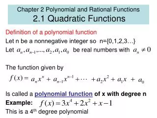
Quadratic functions, f(x)= graph to be a parabola. The vertex of the parabolas is at (h,k) and “a” describes the “steepness” and direction of the parabola given
Minimum (or maximum) function value for a quadratic occurs at the vertex. • If equation is not in standard form, you may have to complete the square to determine the point (h,k). If parabola opens up, f(x) has a min., if it opens down, f(x) has a max. • This parabola opens up with a “steepness” of 2 and the minimum is at (1,1). (graph on next page)
2.3 Polynomial Functions & Their Graphs • Objectives • Identify polynomial functions. • Recognize characteristics of graphs of polynomials. • Determine end behavior. • Use factoring to find zeros of polynomials. • Identify zeros & their multiplicities. • Use Intermediate Value Theorem. • Understand relationship between degree & turning points. • Graph polynomial functions.
The highest degree in the polynomial is the degree of the polynomial. • The leading coefficient is the coefficient of the highest degreed term. • Even-degreed polynomials have both ends opening up or opening down. • Odd-degreed polynomials open up on one end and down on the other end. • WHY? (plug in large values for x and see!!)
Zeros of polynomials • When f(x) crosses the x-axis. • How can you find them? • Let f(x)=0 and solve. • Graph f(x) and see where it crosses the x-axis. What if f(x) just touches the x-axis, doesn’t cross it, then turns back up (or down) again? This indicates f(x) did not change from pos. or neg. (or vice versa), the zero therefore exists from a square term (or some even power). We say this has a multiplicity of 2 (if squared) or 4 (if raised to the 4th power).
Intermediate Value Theorem • If f(x) is positive (above the x-axis) at some point and f(x) is negative (below the x-axis) at another point, f (x) = 0 (on the x-axis) at some point between those 2 pts. • True for any polynomial.
Turning points of a polynomial • If a polynomial is of degree “n”, then it has at most n-1 turning points. • Graph changes direction at a turning point.
Graph, state zeros & end behavior • END behavior: 3rd degree equation and the leading coefficient is negative, so if x is a negative number such as -1000, f(x) would be the negative of a negative number, which is positive! (f(x) goes UP as you move to the left.) and if x is a large positive number such as 1000, f(x) would be the negative of a large positive number (f(x) goes DOWN as you move to the right.) • ZEROS: x = 0, x = 3 of multiplicity 2 • Graph on next page
2.4 Dividing polynomials; Remainder and Factor Theorems • Objectives • Use long division to divide polynomials. • Use synthetic division to divide polynomials. • Evaluate a polynomials using the Remainder Theorem. • Use the Factor Theorem to solve a polynomial equation.
How do you divide a polynomial by another polynomial? • Perform long division, as you do with numbers! Remember, division is repeated subtraction, so each time you have a new term, you must SUBTRACT it from the previous term. • Work from left to right, starting with the highest degree term. • Just as with numbers, there may be a remainder left. The divisor may not go into the dividend evenly.
Remainders can be useful! • The remainder theorem states: If the polynomial f(x) is divided by (x – c), then the remainder is f(c). • If you can quickly divide, this provides a nice alternative to evaluating f(c).
Factor Theorem • f(x) is a polynomial, therefore f(c) = 0 if and only if x – c is a factor of f(x). • If we know a factor, we know a zero! • If we know a zero, we know a factor!
2.5 Zeros of Polynomial Functions • Objectives • Use Rational Zero Thm. to find possible zeros. • Find zeros of a polynomial function. • Solve polynomial equations. • Use the Linear Factorization Theorem to find polynomials, given the zeros. • Use Descartes’s Rule of Signs.
Rational Root (Zero) Theorem • If “a” is the leading coefficient and “c” is the constant term of a polynomial, then the only possible rational roots are factors of “a” divided by factors of “c”. • Example: • To find the POSSIBLE rational roots of f(x), we need the FACTORS of the leading coefficient and the factors of the constant term. Possible rational roots are
How many zeros does a polynomial with rational coefficients have? • An nth degree polynomial has a total of n zeros. Some may be rational, irrational or complex. • Because all coefficients are RATIONAL, irrational roots exist in pairs (both the irrational # and its conjugate). Complex roots also exist in pairs (both the complex # and its conjugate). • If a + bi is a root, a – bi is a root • If is a root, is a root.
Descartes’s Rule of Signs • Depends on the number of sign changes (switching from pos. to neg. or vice versa) • Count sign changes in f(x). # of pos. real zeros is the # of sign changes or an even number less than # of sign changes. • Count sign changes in f(x). # of neg. real zeros is # of sign changes or an even number less than the # of sign changes.
2.6 Rational Functions & Their Graphs • Objectives • Find domain of rational functions. • Use arrow notation. • Identify vertical asymptotes. • Identify horizontal asymptotes. • Use transformations to graph rational functions. • Graph rational functions. • Identify slant (oblique) asymptotes. • Solve applied problems with rational functions.
Vertical asymptotes • Look for domain restrictions. If there are values of x which result in a zero denominator, these values would create EITHER a hole in the graph or a vertical asymptote. Which? If the factor that creates a zero denominator cancels with a factor in the numerator, there is a hole. If you cannot cancel the factor from the denominator, a vertical asymptote exists. • If you evaluate f(x) at values that get very, very close to the x-value that creates a zero denominator, you notice f(x) gets very, very, very large! (approaching pos. or neg. infinity as you get closer and closer to x)
Example • f(x) is undefined at x = 2 • As • Therefore, a vertical asymptote exists at x=2. The graph extends down as you approach 2 from the left, and it extends up as you approach 2 from the right.
What is the end behavior of this rational function? • If you are interested in the end behavior, you are concerned with very, very large values of x. • As x gets very, very large, the highest degree term becomes the only term of interest. (The other terms become negligible in comparison.) • SO, only examine the ratio of the highest degree term in the numerator over the highest degree term of the denominator (ignore all others!) • As x gets large, becomes • THEREFORE, a horizontal asymptote exists, y=3
What if end behavior follows a line that is NOT horizontal? • Using only highest-degree terms, we are left with • This indicates we don’t have a horizontal asymptote. Rather, the function follows a slanted line with a slope = 4. (becomes y=4x as we head towards infinity!) • To find the equation of the slant asymptote, proceed with long division, as previously done. The quotient is the slant (oblique) asymptote. For this function, y = 4x – 11/2 • NOTE: f(x) also has a vertical asymptote at x=1.
What is the equation of the oblique asymptote? • y = 4x – 3 • y = 2x – 5/2 • y = 2x – ½ • y = 4x + 1
2.7 Polynomial & Rational Inequalities • Objectives • Solve polynomial inequalities. • Solve rational inequalities. • Solve problems modeled by polynomial or rational inequalities.
Solving polynomial inequalities • Always compare the polynomial to zero. • Factor the polynomial. We are interested in when factors are either pos. or neg., so we must know when the factor equals zero. • The values of x for which the factors equal zero provide the cut-offs for regions to check if the polynomial is pos. or neg.
(x – 3)(x + 1)(x – 6) < 0 • In order for the product of 3 terms to be less than zero (negative), either all 3 terms must be neg. or exactly 1 of them be neg. • The 3 “cut-off” values are x = 3,-1,6 • The 3 cut-off values create 4 intervals along the x-axis: • Pick a point in each interval & determine if that value for x would make all 3 factors neg. or exactly 1 negative. If so, the function is < 0 on that interval. • x<-1, f(x) < 0 -1<x<3, f(x) > 0 • 3<x<6, f(x)< 0 x>6, f(x) > 0 • Solution: {x: x < -1 or 3 < x < 6}
Given the following graph of f(x), give interval notation for x-values such that f(x)>0.
Solving rational inequalities • VERY similar to solving polynomial inequalites EXCEPT if the denominator equals zero, there is a domain restriction. The function COULD change signs on either side of that point. • Step 1: Compare inequality to zero. (add constant to both sides and use a common denominator to have a rational expression) • Step 2: Factor both numerator & denominator to find “cut-off” values for regions to check when function becomes positive or negative.
2.8 Modeling Using Variation • Objectives • Solve direct variation problems. • Solve inverse variation problems. • Solve combined variation problems. • Solve problems involving joint variation.
Direct variation • y varies directly as x (y is directly proportional to x) if y = kx. • k is the constant of variation (constant of proportionality) • This is the graph of a linear function with slope = m, crossing through the origin. • Example: You are paid $8/hr. Thus, pay is directly related to hours worked: pay=8(hours worked)
Direct variation COULD involve an nth power of x (no longer linear) • Still involves a constant of proportionality • y is directly proportional to the nth power of x.
Inverse Variation • As x gets bigger, y gets smaller • As x gets smaller, y gets bigger
Combined Variation Problem • y is impacted by TWO variables in TWO different ways. One variable causes y to get bigger, while the other variable causes it to become smaller. • As x gets bigger, y gets bigger, but as z gets bigger, y gets smaller. • k must take into account both influences

