Download
1 / 35
350 likes | 525 Vues
Beam Loss Monitoring. S.Mallows , E.B.Holzer , J. van Hoorne M.Zingl , L.Devlin. Overview. CLIC BLM Considerations Machine Protection Strategy Expected Beam Losses in the 2 beam modules Ionization Chambers as a Suitable Baseline Technology Choice Dynamic Range, Sensitivity

E N D
Beam Loss Monitoring S.Mallows, E.B.Holzer, J. van HoorneM.Zingl, L.Devlin
Overview • CLIC BLM Considerations • Machine Protection Strategy • Expected Beam Losses in the 2 beam modules • Ionization Chambers as a Suitable Baseline Technology Choice • Dynamic Range, Sensitivity • Investigation of Cherenkov Fibers as an Alternative Technology Choice • Model for light yield • Longitudinal Position Resolution with Fiber • Radiation Hardness Sophie Mallows, CLIC Workshop 2013
Beam Loss Monitors • A BLM typically sits outside the vacuum chamber and measures the secondary particle shower resulting from beam loss • Used for machine protection and beam diagnostics Sophie Mallows, CLIC Workshop 2013
CLIC Machine Protection Strategy • Based on Passive protection and a “Next cycle permit” • Primary role of the BLM system as part of the Machine Protection System is to prevent subsequent injection into the Main Beam linac and the Drive Beam decelerators when potentially dangerous beam instabilities are detected • Option of CLIC at 100Hz Minimum Response time <8ms required by BLMs to allow post pulse analysis Sophie Mallows, CLIC Workshop 2013
Standard Operational Losses • Limits in the Two Beam Modules • Activation(Residual Dose Rates – Access Issues) • Damage to beamline components • Damage to electronics (SEE’s, Lattice Displacement, Total Ionizing Dose) • Beam dynamics considerations (luminosity losses due to beam loading variations) • 10-3 of full intensity of the Main Beam over 21km linac • 10-3 of full intensity of the Drive Beam over ~875m decelerator • How are the losses distributed over the length of the decelerator? Recent discussions with Guido Sterbini, JakobEsbergto define estimation Sophie Mallows, CLIC Workshop 2013
Loss Scenarios • Dust particles falling into beam (‘UFOs’), misalignments, etc • Possible failure scenarios in two beam modules under investigation (PLACET Simulations, CERN: TE-MPE-PE) • Consider destructive limits (fraction of beam hitting single aperture). • [ Destructive potential: notdetermined by Beam Power but by Power Density, i.e. Beam Charge/ Beam Size • Main Beam (damping ring exit) 10000 * safe beam • 0.01 % of bunch – 1.16e8 electrons • Drive Beam decelerators 100 * safe beam • 1.0% of a bunch train 1.53e12 electrons Sophie Mallows, CLIC Workshop 2013
BLM Requirements (as specified in CDR ) Dynamic Range - Upper Limit • Detect onset of Dangerous losses • FLUKA: Loss at single aperture • Upper Limit of Dynamic Range, 10% destructive loss (desirable) • 0.1% DB bunch train, 0.001% bunch train MB Sensitivity • Standard Operational Losses • FLUKA: Loss distributed longitudinally • Lower Limit of Dynamic Range: 1% loss limit for beam dynamics requirements • 10-5 train distributed over MB linac, DB decelerator [NB! Assumed uniform losses along decelerators/linacs ] • Example: Spatial distribution of absorbed dose for maximum operational losses distributed along aperture (DB 2.4 GeV) Scaling: 10-3 bunch train/875m • Example: Spatial distribution of absorbed dose resulting from loss of 0.01% of 9 GeV MB bunch train at a single aperture Sophie Mallows, CLIC Workshop 2013
Ionization Chambers for TBMs • Ionization Chambers fulfill necessary requirements for machine protection and diagnostics • LHC Ionization Chamber + readout electronics • Dynamic Range 105 (106 under investigation) • Sensitivity 7e10-9Gy • See: CLIC CDR • But: Large number of BLMs required – cost concern • >45 thousand quadrupolemagnets over 42 km (41.5 thousand in the decelerator modules) • Investigate Alternative Technologies for the Two Beam Modules in the post CDR phase • Technologies that cover a large distance along the beamline • E.g. long ionization chambers, optical fibers Sophie Mallows, CLIC Workshop 2013
Cherenkov Fiber BLM • Advantages • Only sensitive to charged particles Insensitive to gamma radiation (and therefore background from activation) • Very small, diameter <1mm • Quartz is radiation hard (c.f. scintillating fibers) • Insensitive to magnetic field, temperature fluctuations. • Disadvantages • Lower Sensitivity c.f. scintillating fibers (which give about 1000 times more light output) • A low proportion of the produced Cherenkov light reaches fiber end face • Angular dependent response • Radiation Effects: Radiation Induced Attenuation Sophie Mallows, CLIC Workshop 2013
Cherenkov Fiber BLM • When a charged particle with v>c enters the fiber, photons are produced along Cherenkov cone of opening angle • Detect photons that are produced, trapped and propagate to the fiber end face and exit in the nominal acceptance cone • ‘Typical’ Fiber BLM: detect upstream photons • α - angle between particle track and fiber axis • β - particle velocity nominal acceptance cone t= Δ z/c t=0 c t=Δz/c + Δ z/(c.2/3) 2/3c 2/3c 2/3c photon detector fiber Sophie Mallows, CLIC Workshop 2013
Light Yield in Fiber • Model to calculate probability as function of incident particle velocity and angle: • Pt:trapping produced photons inside the fiber • Pe:photons exiting at the fiber end face • Pe,a: photons exiting within ‘acceptance’ cone • Test beam measurements with 120 GeV protons to compare with model: • Angular dependency • Diameter dependency • Time dispersion J. van Hoorne • α - angle between particle track and fiber axis;β - particle velocity; Analytical expression from: S.H. Law et al., Appl. Opt. 45(36):9151-9159, 2006 Results Angular dependency of the photon yield in a fiber (dfiber=0.365mm, NA=0.22, Lfiber~4m) Sophie Mallows, CLIC Workshop 2013
Cherenkov Fibers as a BLM for CLIC • FLUKA simulations • Score angular and velocity distribution of charged particles at fiber locations and use asinput to determine the photon signal • Initial study in post CDR phase indicated fibers as feasible option in terms of sensitivity and dynamic range for drive beams (IPAC, 2011) • Tables [Scaling: Loss assumptions as specified in CDR] Blue lines indicate location of boundaries for scoring particle shower distribution (5cm high) e+/e- fluence per primary electron impacting at single location Sophie Mallows, CLIC Workshop 2013
Attenuation • In the UV/VIS range (λ=300 to 700nm) the dominant attenuation effect in optical fibers is Rayleigh Scattering; attenuation coefficient is proportional to λ-4. • Therefore, for fibers longer than 200m the blue/green part of the radiation spectrum becomes insignificant Fibers should not be longer than ≈100m Photon spectra after propagation through quartz fiber Example of photon efficiency of a Hamamatsu MPPC Additional absorption bands from impurities Photon detection efficiency of MPPC [%] photon yield [a.u.] Sophie Mallows, CLIC Workshop 2013
Radiation Effects in Multimode Fibers • All properties are changed (some only at high doses) • Including Refractive Index, bandwidth, and mechanical properties • Most Important: Increase in attenuation (Radiation Induced Attenuation -RIA) • Depends on radiation environment , fiber materials and manufacturing conditions • Some general rules of thumb for rad hardness: Fluorine, not phosphorus-doped, High OH content, J.Kuhnhenn, 7th DTANET Topical Workshop • Careful selection and radiation testing is necessary J.Kuhnhenn • Example: Coating /CCDR influence on RIA in Step Index Fibers Sophie Mallows, CLIC Workshop 2013
Radiation Hardness Cherenkov Fibers • CLIC radiation environment: Conservative estimates - 50kGy/yrnear beam lines. • Better estimate of loss distribution along drive beam linacs might reduce this. • Rad Hard Fibers • CMS quartz calorimeter fibers: some tested ok up to 22 MGy(P. Gorodetzky et al., NIMA 361:161-179, 1995; and V. Hagopian, CMS-CR-1999-002) (wavelength dependence!) • Kuhnhenn et al, RADECS 2005 • Perform tests at FrauenhoferInstitute (early 2013) RIA at approx. 450nm for up to at least 10 kGy on 2 fibers: Heraeuspreform(as installed at CTF-3), Ultrasol-fibers(Solarisation resistant) • Radiation Induced Attenuation for variousfibers measured at 660nm Sophie Mallows, CLIC Workshop 2013
Longitudinal Resolution Fibers • Required resolution • Machine protection purposes • Detecting the integrated loss signal is sufficient • Beam diagnostics • What is the desired longitudinal resolution ? • (for which loss scenario) • Quadrupolespacing is ~1m in drive beams • Achievable resolution • Single short pulses: Fiber coupled to SiPM, 250MS/s ADC~ 50cm • What is the achievable resolution with long bunch trains ? • Drive beam 244ns or 80m • Main beam 156ns or 50m c bunch train fiber 2/3c 2/3c photon detector photondetector Sophie Mallows, CLIC Workshop 2013
Single Bunch Trains • Dispersion effects: • Arrival time depends on photon trajectory in fiber • Highly skewed rays can be blocked by collimation • Single Bunch Resolution: • Arrival time distribution of photons simulated for drive beam 2.4 GeVloss at 50m along 100m fiber • Rising edge of the photon signal < 2 ns M.Zingl Sophie Mallows, CLIC Workshop 2013
Loss Scenarios - Example Simulation • Loss at a single location Sophie Mallows, CLIC Workshop 2013
Loss Reconstruction • Drive Beam 2.4 GeV • Naïve (simple) back projection • Bars indicate the full extent of the rise • Furthest point is < 50cm from the real loss location Sophie Mallows, CLIC Workshop 2013
Multi-bunch Trains • In general it is not possible to reconstruct an arbitrary loss pattern (in position and time) • But, only few different loss patterns are to be expected 1. Single or multiple individual loss locations • Constant losses in time, i.e. obstructions • Variation in time, i.e. interaction with “dust particles” 2. Losses building up along the train, starting at a certain position • bunch number (i.e. long range or resistive wall wake fields) • Combined with aperture limitation 3. Constant losses • Beam gas scattering • As a function of distance along decelerator • optics mis-match 4. Equipment failures 5. Others? Sophie Mallows, CLIC Workshop 2013
Space Time Diagrams • Loss at single location, Loss at two locations • Location of loss determined from signal rise time • Upstream signal gives a better resolution and real time sequence of losses Sophie Mallows, CLIC Workshop 2013
Current investigations • Can all the expected loss scenarios be distinguished? • With what resolution ? • Do all scenarios require the same longitudinal resolution? • Could additional measurements improve resolution? • E.g. fast, localised detector every ≈ 20 - 100 m to measure loss structure within the train (e.g. diamond BLM) Sophie Mallows, CLIC Workshop 2013
Current Investigations • Integration into 2 Beam Modules • Best location for fibers • Measurements at CTF-3 • ‘Catalogue’ of simulations for all expected loss scenarios • E.g. UFO 100 um thick , 2.4 GeV Drive Beam Sophie Mallows, CLIC Workshop 2013
First Measurements at TBL - Fiber Signal Layout: SiPMs 75m 25m Ceiling Upstream Photons TBL FIBER 28m Downstream Photons e- Faisceau: TBL Subtraction of ‘Background’ Raw Signals Sophie Mallows, CLIC Workshop 2013
Summary • Ionization chambers suitable (but expensive) baseline technology choice • Cherenkov fibers seem feasible alternative for CLIC drive beams • Ongoing investigation of loss scenarios (CLIC) and corresponding simulations. • Ongoing measurements at CTF3 • Determination achievable longitudinal resolution to allow comparison with other technologies Sophie Mallows, CLIC Workshop 2013
Spare SLIDES Sophie Mallows, CLIC Workshop 2013
Photon Detector • What is an SiPM? • Silicon Photomultiplier - array of APDs connected in parallel • Each pixel is a p-n junction in self-quenching Geiger mode • Reverse Bias causes APD breakdown • Electron avalanche: PMT-like gain • Pixels are equally sized and independent • Analog output – Signal is sum of fired pixel signals • SiPM Advantages: • Compact and light • Low operating voltage (20-100V) • Simple FE electronics • Fast signal (~1ns) • Cheap • Suitability Dynamic range, radiation hardness Sophie Mallows, CLIC Workshop 2013
Cross Talk Issues • Desirable to distinguish between a failure loss from each of the beams • Spatial Distribution of prompt Absorbed Dose (Gy) from FLUKA Simulations: • Loss of 1.0% in DB provokes similar signal as a loss of 0.01% of MB in region close to MB quadrupole. • NOT a Machine Protection Issue – Dangerous loss would never go unnoticed • Compare signals from both fibers each side to distinguish Main and Drive Beam losses. Destructive DB 1.0% of bunch train hits single aperture restriction Destructive MB 0.01% of bunch train hits single aperture restriction Workshop on Machine Protection 6-8th June 2012
Drive Beam Sophie Mallows 0.24 GeV 2.4 GeV Same FLUKA - Particle fluence spectra after quadrupoles.
Main Beam Sophie Mallows 9 GeV 1.5 TeV Particle fluence spectra after quadrupoles.
Radiation Levels Annual Absorbed Dose from maximum permissible losses in Drive Beam at 2.4 GeV (assuming 180 days running at nominal intensity ) 2 1 Workshop on Machine Protection 6-8th June 2012
Radiation Induced Attenuation Wavelength Dependence Core Doping • Example Ge doped fiber • lfiber 100m, for λ 830nm Manufacturing Manufacturing (Coating/CCDR ) • Graded Index Fibers • Step Index Fibers Sophie Mallows, CLIC Workshop 2013
BLM Installation (ACEMs) 16-AS 15-AS 12-AS 11-AS 08-AS 07-AS 04-AS 03-AS e- CB.QF940 CB.QF900 CB.QF840 CB.QF800 CB.QF740 CB.QF700 CB.QF640 CB.QF600 CB.QF540 CB.QF500 CB.QF440 CB.QF400 CB.QF340 CB.QF300 CB.QF240 CB.QF200 ACEM installed Sophie Mallows, CLIC Workshop 2013
Loss Scenario – Example Simulations • Impact Points (UFO Simulation) Sophie Mallows, CLIC Workshop 2013
CDR Summary Table Sophie Mallows, CLIC Workshop 2013