Equivalent Quadratic Forms - Lesson 7.2
Learn about equivalent forms of quadratic functions, including the vertex form and factored form. Practice finding zeros and graphing parabolas.

Equivalent Quadratic Forms - Lesson 7.2
E N D
Presentation Transcript
EquivalentQuadratic Forms Lesson 7.2
In Lesson 7.1, you were introduced to polynomial functions, including 2nd-degree polynomial functions, or quadratic functions. • The general form of a quadratic function is y=ax2+bx+c. • In this lesson you will work with two additional, equivalent forms of quadratic functions.
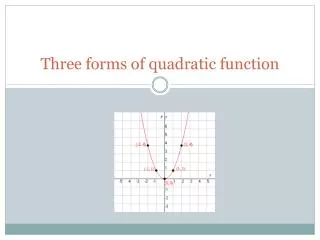
Recall from Chapter 4 that every quadratic function can be considered as a transformation of the graph of the parent function y =x2 . • A quadratic function in the form identifies the location of the vertex, (h, k), and the horizontal and vertical scale factors, a and b.
Example A • Find the horizontal and vertical scale factors of the parabola at the right with vertex (4,2) and write its equation. Then rewrite the equation with a single scale factor.
Example A • If you consider the point (7,4) to be the image of the point (1,1) on the graph of y=x2, the horizontal scale factor is 3 and the vertical scale factor is 6. So the quadratic function is
To rewrite the equation with a single scale factor, first move the denominator out of the parentheses, which gives the equation • This equation is equivalent to • This form combines the original horizontal and vertical scale factors into a single vertical scale factor, 2/3 and shows the vertex (4,2).
This new form, , is called the vertex form of a quadratic function because it identifies the vertex, (h, k), and a single vertical scale factor, a.
The y-coordinate of any point along the x-axis is 0, so the y-coordinate is 0 at each x-intercept. • For this reason, the x-intercepts of the graph of a function are called the zeros of the function. You will use this information and the zero-product property to find the zeros of a function without graphing.
Example B • Find the zeros of the function y =1.4(x-5.6)(x+3.1). • The zeros will be the x-values that make y equal 0. • First, set the function equal to zero.0 =1.4(x-5.6)(x+3.1) • Because the product of three factors equals zero, the zero-product property tells you that at least one of the factors must equal zero. • 1.4=0 (not possible) or x-5.6=0 (x=5.6) or x+3.1= 0 (x=-3.1) • That means the zeros of the function y =1.4(x-5.6)(x+3.1) are x=5.6 and x=-3.1.
Use your graphing calculator to check your work. You should find that the x-intercepts of the graph of y =1.4(x-5.6)(x+3.1). are 5.6 and -3.1.
Example C • Consider the parabola at right. • Write an equation of the parabola in vertex form. The vertex form is y =(x-1)2-4
Example C • Consider the parabola at right. • Write an equation of the parabola in factored form. The x-intercepts are 1 and 3, so the factored form is y= a(x+1)(x-3). To verify that the scale factor, you can solve for it analytically. Substitute the coordinates of another point on the parabola such as (2, 3) into the equation for x and y.
Example C • Consider the parabola at right. • Show that both equations are equivalent by converting them to general form.
Rolling Along Procedural Note Prop up one end of the table slightly. Place the motion sensor at the low end of the table and aim it toward the high end. With tape or chalk, mark a starting line 0.5 m from the sensor on the table.
Rolling Along • Practice rolling the can up the table directly in front of the motion sensor. Start the can behind the starting line. Give the can a gentle push so that it rolls up the table on its own momentum, stops near the end of the table, and then rolls back. Stop the can after it crosses the line and before it hits the motion sensor.
Set up your calculator to collect data for 6 seconds. When the sensor begins, roll the can up the table. • The data collected by the sensor will have the form (time, distance). Adjust for the position of the starting line by subtracting 0.5 from each value in the distance list. • Let x represent time in seconds, and let y represent distance from the line in meters. Draw a graph of your data. What shape is the graph of the data points? • What type of function would model the data? Use finite differences to justify your answer.
The shape of the graph is parabolic. A quadratic function would model these data. The second differences, D2, are almost constant around 0.06, which implies that a quadratic model is appropriate.
Mark the vertex and another point on your graph. Approximate the coordinates of these points and use them to write the equation of a quadratic model in vertex form. vertex: (3.2, 4.757); point: (5.2, 1.397); Horizontal stretch: 5.2-3.2 or 2 Vertical stretch: 1.397 -4.757or -3.36
From your data, find the distance of the can at 1, 3, and 5 seconds. Use these three data points to find a quadratic model in general form. (1, 1.046), (3, 4.756), and (5, 1.993); 1.046=a(1)2 + b(1) +c 4.756=a(3)2 + b(3) +c 1.993=a(5)2 + b(5) +c a= -0.81, b= 5.09 and c = -3.24 Y= -0.81x2 +5.09x -3.24
Mark the x-intercepts on your graph. Approximate the values of these x-intercepts. Use the zeros and the value of a from Step 5 to find a quadratic model in factored form. Zeros: (0.7, 0) and (5.6, 0); Y= -0.84(x-0.7)(x-5.6)
Verify by graphing that the three equations in the last three steps are equivalent, or nearly so. Write a few sentences explaining when you would use each of the three forms to find a quadratic model to fit parabolic data. y= -0.81x2 +5.09x -3.24 y= -0.84(x-0.7)(x-5.6)