Download
1 / 26
260 likes | 290 Vues
Explore the latest developments in numerical polynomial algebra and algebraic geometry, including factorization, GCD computation, multiplicity structure identification, and matrix computations.

E N D
Matrix Computationin Numerical Polynomial Algebraand Algebraic Geometry Zhonggang Zeng Northeastern Illinois University Linear and Numerical Linear Algebra: Theory, Method, and Applications August 14, 2009, De Kalb, (supported in part by NSF under Grant DMS-0715137)
Sample problem: Factor with inexact coefficients (a.k.a. root-finding problem) 1
Sample problem: Factor with inexact coefficients (a.k.a. root-finding problem) Matlab factorization Numerical irreducible factorization: >> [F,res,fcnd] = uvFactor(f,1e-10,1); THE CONDITION NUMBER: 914.329 THE BACKWARD ERROR: 5.71e-015 THE ESTIMATED FORWARD ROOT ERROR: 1.04e-011 FACTORS ( x - 3.999999999999990 )^20 ( x - 3.000000000000008 )^40 ( x - 1.999999999999998 )^60 ( x - 1.000000000000000 )^80 Z. Zeng, TOMS 2004, Math Comp 2005, ISSAC 2009
(Kaltofen, Problem 1 in “Challenges of symbolic computation”, 2000) Sample problem: Factor a multivariate polynomial Factorization fails 3
approximation A factorable polynomial irreducible Factoring a multivariate polynomial: Question: How to factor a multivariate polynomial approximately? 4
What’s the multiplicity of the function f(x) =x3– 6 x cos(x2) + 6 sin(x) at the zero x* = 0? Textbooks say: 0 = f(x*) = f’(x*) = f”(x*) = f’’’(x*) = f(4)(x*) f(5)(x*) = 366 0 Multiplicity = 5 Sample problem: What is the multiplicity of the nonlinear system at the zero 5
Differential orders 6 depth = 6 5 4 3 2 1 0 breadth=2 Example: Considerthe multiplicity structureof at an isolated multiple zero (0,0) • Multiplicity = 12 • Perturbed system has 12 zeros near (0,0) • Hilbert function = {1,2,3,2,2,1,1,0,…} • Dual spaceD(0,0) (F) spanned by Multiplicity is not just a number! Question: How to identify the multiplicity structure? 6
Symbolic computation has thrived for decades in polynomial algebra and algebraic geometry • Gröbner basis • Polynomial factorization • Computer Algebra Systems (Maple, Mathematica, etc) Bruno Buchberger with limitations. 7
Pioneer works in numerical polynomial algebra and algebraic geometry (incomplete list) • Homotopy method for solving polynomial systems • (Li, Sommese, Wampler, Verschelde, …) • Numerical Algebraic Geometry • (Sommese, Wampler, Verschelde, …) • Numerical Polynomial Algerba • (Stetter) A frontier in scientific computing, and may be the beginning of Numerical Nonlinear Algebra 8
Recent progress in numerical polynomial algebra • Solving polynomial systems (Li, Sommese, Verschelde, …) • Approximate multiple roots/factorization (Zeng 2005, 2009) • Approximate GCD(Zeng-Dayton 2004) • Approximate irreducible factorization(Sommesse-Wampler-Verschelde 2003, Gao et al 2003, 2004, Zeng in progress) • Computing multiplicity structure(Dayton-Zeng 05, Bates-Peterson-Sommese ’06) • Polynomial elimination(Zeng, 2008) • Feedback from num. polyn. algebra to numerical linear algebra: • Approximate rank/kernel (Li,Zeng 2005, Lee, Li, Zeng 2009) • Approximate Jordan Canonical Form (Zeng-Li in progress) 9
Among many challenges in numerical polynomial algebra: • Regularizing ill-posed problems for approximate solutions • numerical polynomial algebra via matrix computations • Handling huge matrices with subspace strategies 10
after formulating the approximate solution to problem P within e Stage I: Find the pejorative manifold P of the highest codimension s.t. P P S Stage II: Find/solve problem Q such that Q The two-staged strategy by numerical matrix computations by the Gauss-Newton iteration Exact solution of Q is the approximate solution of P within e which approximates the solution of S where P is perturbed from 11
Example: For polynomial with (inexact ) coefficients in hardware precision Matlab factorization Approximate irreducible factorization: >> [F,res,fcnd] = uvFactor(f,1e-10,1); THE CONDITION NUMBER: 914.329 THE BACKWARD ERROR: 5.71e-015 THE ESTIMATED FORWARD ROOT ERROR: 1.04e-011 FACTORS ( x - 3.999999999999990 )^20 ( x - 3.000000000000008 )^40 ( x - 1.999999999999998 )^60 ( x - 1.000000000000000 )^80 Zeng, 2005, 2009 12
How to identify the solution structure? Answer: Matrix computations 13
Matrix computation is not always good. Is this matrix nonsingular? (polynomial long division) The condition number ≥ 10n Distance to singularity 1/10n The error in data can be magnified by 10n times into the solution z. “Life is too short for long division” anyway. 14
If then The linear transformation has a nontrivial kernel: Matrix for L is rank-deficient Example: How to determine the GCD structure 15
Moreover xj xj [ ] xj The linear transformation On the vector space Has the kernel Linear transformation L Sylverster matrix S(f,g) James J. Sylvester Numerical rank-deficiency = degree of the approx. GCD 16
Namely, (p, q) satisfy linear equation Case study: How to solve Find such that --- leading to matrix rank/kernel problem(Zeng, TCS 2008) 17
= = Multivariate factorization structure: Matrix computations! For any polynomial f(x,y) Assume f = f1 f2 f3 with distinct factors f1, f2, and f3 The equation has three solutions # of factors = # of solutions to 18
A squarefree polynomial f C[x,y] of bidegree [m,n] has k distince factors the homogeneous linear equation has k linearly independent solutions (g,h) of bidegrees deg(g) [m-1,n], deg(h) [m,n-1]. Irreducibility condition (Ruppert ‘99, and Gao ‘03, Kaltofen-May ’03,Gao-Kaltofen-May-Yang-Zhi’04) is a linear transformation corresponding to a matrix Rf Rank-deficiency = # of irreducible factors a random nulvector of matrix Rf corresponds to g = l1f1,x f2 … fk + … + lkf1 f2 … fk,x h = l1f1,y f2 … fk + … + lkf1 f2 … fk,y 19
GCD( f, g -li fx ) = fi for i = 1, 2, …, k Namely, Takingg = l1f1,x f2 f3 + l2f1, f2x f3 + l3f1 f2 f3,x( f = f1 f2 f3) g -l1 fx= (l2 -l1) f1 f2,x f3 + (l3 - l1) f1 f2 f3,x Let deg( fi ) = [mi,, ni ]. Then, for fixed random ( x*, y* ), the Sylvester matrices S(f(, y*),g (, y*)-li fx (, y*) ) is of nullity mi, S(f(x* ,),g (x* ,)-li fx (x* ,) ) is of nullity ni, li is an eigenvalue of geometric multiplicity mi the matrix pencil S(f(, y*),g (, y*) )-lS( 0, fx (, y*) ) A-lB Numerical polynomial factorization can be done by matrix computation! 20
Differential orders 6 depth = 6 5 4 3 2 1 0 breadth=2 Example: Considerthe multiplicity structureof at an isolated multiple zero (0,0) • Multiplicity = 12 • Perturbed system has 12 zeros near (0,0) • Hilbert function = {1,2,3,2,2,1,1,0,…} • Dual spaceD(0,0) (F) spanned by Case study: How to identify the multiplicity structure of a nonlinear system? 21
Univariate case: x* is m-fold if 0 = f(x*) = f’(x*) = … = f(m-1)(x*) and f(m)(x*)≠0 A (differential) functional at zero evaluated at linear combination of = the # of linearly Independent functionals vanishing on ideal I Multivariate case: Dual space defines the multiplicity structure at 22
Fundamental Theorems of the multiplicity: Local Finiteness Theorem: The zero is isolated iff the multiplicity is finite. Perturbation Invariance Theorem: The number of zeros is invariant counting multiplicities under small perturbation to the system. Multiplicity Consistence Theorem: The intersection multiplicity = dual multiplicity. Depth Deflation Theorem: Multiple zeros can be accurately computed by a deflation method, with the number of deflation steps bounded by the depth of the zero. (Dayton, Li, and Zeng, Multiple zeros of nonlinear systems, 2009) Joint work with 23
Multiplicity matrices and nullspaces 24