Download
1 / 39
390 likes | 569 Vues
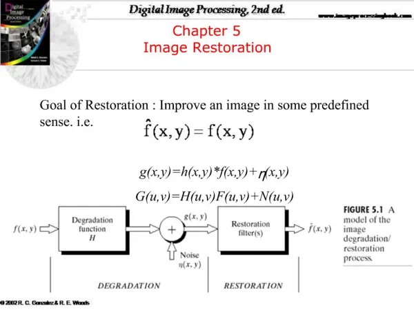
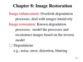
Chapter 8: Image Restoration 8.1 Introduction. Image restoration concerns the removal or reduction of degradations that have occurred during the acquisition of the image

E N D
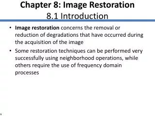
Chapter 8:Image Restoration8.1 Introduction • Image restoration concerns the removal or reduction of degradations that have occurred during the acquisition of the image • Some restoration techniques can be performed very successfully using neighborhood operations, while others require the use of frequency domain processes Ch8-p.191
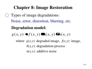
8.1.1 A Model of Image Degradation • f(x, y) : image h(x, y) : spatial filter • Where the symbol * represents convolution • In practice, the noise n(x, y) must be considered Ch8-p.191
8.1.1 A Model of Image Degradation • We can perform the same operations in the frequency domain, where convolution is replaced by multiplication • If we knew the values of H and N, we could recover F by writing the above equation as this approach may not be practical Ch8-p.192
8.2 Noise • Noise—any degradation in the image signal caused by external disturbance • These errors will appear on the image output in different ways depending on the type of disturbance in the signal • Usually we know what type of errors to expect and the type of noise on the image; hence, we can choose the most appropriate method for reducing the effects Ch8-p.192
8.2.1 Salt and Pepper Noise • Also called impulse noise, shot noise, or binary noise, salt and pepper degradation can be caused by sharp, sudden disturbances in the image signal • Its appearance is randomly scattered white or black (or both) pixels over the image Ch8-p.192
>> imshow(t) >> figure, imshow(t_sp) FIGURE 8.1 Ch8-p.193
8.2.2 Gaussian Noise • Gaussian noise is an idealized form of white noise, which is caused by random fluctuationsin the signal • If the image is represented as I, and the Gaussian noise by N, then we can model a noisy image by simply adding the two Ch8-p.193
8.2.3 Speckle Noise • Speckle noise (or more simply just speckle) can be modeled by random values multiplied by pixel values • It is also called multiplicative noise • imnoise can produce speckle Ch8-p.194
FIGURE 8.2 Ch8-p.194
8.2.4 Periodic Noise Ch8-p.195
8.3 Cleaning Salt and Pepper Noise • Low-Pass Filtering Ch8-p.196
8.3.2 Median Filtering Ch8-p.197
FIGURE 8.6 Ch8-p.198
FIGURE 8.7 Ch8-p.198
8.3.3 Rank-Order Filtering • Median filteringis a special case of a more general process called rank-order filtering • A mask as 3×3 cross shape 0 1 0 1 1 1 0 1 0 Ch8-p.199
8.3.4 An Outlier Method • Applying the median filter can in general be a slow operation: each pixel requires the sorting of at least nine values • Outlier Method • Choose a threshold value D • For a given pixel, compare its value p with the mean m of the values of its eight neighbors • If |p − m| > D, then classify the pixel as noisy, otherwise not • If the pixel is noisy, replace its value with m; otherwise leave its value unchanged Ch8-p.199
FIGURE 8.8 Ch8-p.200
FIGURE 8.9 Ch8-p.201
8.4 Cleaning Gaussian Noise • Image Averaging • suppose we have 100 copies of our image, each with noise • BecauseNiis normally distributed with mean 0, it can be readily shown that the mean of all the Ni’s will be close to zero The greater the number of Ni’s; the closer to zero Ch8-p.202
FIGURE 8.10 Ch8-p.203
8.4.2 Average Filtering Ch8-p.203
8.4.3 Adaptive Filtering • Adaptive filters are a class of filters that change their characteristics according to the values of the grayscales under the mask • Minimum mean-square error filter • The noise may not be normally distributed with mean 0 Ch8-p.204
8.4.3 Adaptive Filtering • Wiener filters (wiener2) Ch8-p.205
FIGURE 8.12 Ch8-p.206
FIGURE 8.13 Ch8-p.206
8.5 Removal of Periodic Noise Ch8-p.207
FIGURE 8.15 • BAND REJECT FILTERING Ch8-p.208
FIGURE 8.16 • NOTCH FILTERING Ch8-p.209
8.6 Inverse Filtering Ch8-p.210
FIGURE 8.18 cutoff radius: 60 Ch8-p.211
FIGURE 8.18 cutoff radius: 80 cutoff radius: 100 Ch8-p.212
FIGURE 8.19 d= 0.005 Ch8-p.213
FIGURE 8.19 d = 0.002 d = 0.001 Ch8-p.213
8.6.1 Motion Deblurring Ch8-p.214
8.6.1 Motion Deblurring • To deblur the image, we need to divide its transform by the transform corresponding to the blur filter • This means that we first must create a matrix corresponding to the transform of the blur Ch8-p.215
FIGURE 8.21 Ch8-p.215
8.7 Wiener Filtering Ch8-p.216
FIGURE 8.22 K = 0.001 Ch8-p.217
FIGURE 8.22 K = 0.0001 K = 0.00001 Ch8-p.217