Download
1 / 77
810 likes | 1.15k Vues
Scheduling of Wafer Fabrication Facilities using Evolutionary Algorithms. Tsung-Che Chiang Department of Computer Science and Information Engineering National Taiwan Normal University 2010.11.04. Outline. Introduction Wafer fab scheduling Evolutionary algorithms (EA)

E N D
Scheduling of Wafer Fabrication Facilities using Evolutionary Algorithms Tsung-Che Chiang Department of Computer Science and Information Engineering National Taiwan Normal University 2010.11.04
Outline • Introduction • Wafer fab scheduling • Evolutionary algorithms (EA) • Six ways of applying EAs to fab scheduling • Conclusions
What’s Scheduling? • A task of allocating resources over time to requests under given constraints such that certain objectives are satisfied or optimized. • In a production system, • resources refer to machines, workers, vehicles, etc. • requests refer to jobs • objectives include work-in-process (WIP) level, on-time delivery (OTD) rate, etc. • A task of allocating resources over time to requests under given constraints such that certain objectives are satisfied or optimized.
schedule 1 time schedule 2 time due dates Single Machine Scheduling • Task: job sequencing
Parallel Machine Scheduling • Tasks: machine assignment & job sequencing schedule 1 time schedule 2 time due date (all the same)
Job Shop Scheduling • Task: job sequencing on each machine • operation precedence • dynamic arrival of jobs M1 M2 M3 M4 M1 M2 M3 M4 M1 M4 M3 M2 M2 M1 M4 M3
Flexible Job Shop Scheduling • Tasks: machine assignment & job sequencing • Machines in a stage might not be identical. S1 S2 S3 S4 M1 M2 M3 M4 M1 M4 M3 M2 M2 M1 M4 M3
Wafer Fab Scheduling • A wafer fab can be regarded as a large-scale flexible job shop with additional intricacies: • batch machines • sequence dependent setup • dynamic arrival of customer orders • machine breakdown & maintenance
batch ID lot size batch forming batch sequencing Wafer Fab Scheduling • Batch machines • batch forming • batch sequencing
Lot2 needs to wait. Processing of Lot1 Lot1 needs to wait. Processing of Lot1 & Lot2 Wafer Fab Scheduling • Batch machines • start or wait Lot2 time Lot1 t0 t1 Lot2 time Lot1 t0 t1
Wafer Fab Scheduling • Sequence dependent setup (SDS) • fixture changing • program loading • parameter tuning • etc. Setup is unproductive. time
Wafer Fab Scheduling • Wafer fab is a very complex system, and optimal scheduling is almost impossible. • A common practice is to do scheduling by real-time dispatching.
cycle-time-based • FCFS (first-come-first-serve) • SPT pj • SRPT rj t: system time dj: due date pj: processing time due-date-based • EDD dj • CR (dj – t)/rj • SLACK dj – t – rj • ATC rj: remaining processing time Rule-based Dispatching queue
Rule-based Dispatching • Some advanced dispatching rules Kim et al. 2001 Pfund et al. 2008
Rule-based Dispatching • Questions • How can we generate a good dispatching rule? • If the rule has parameters, how can we optimize them? • Can we combine different rules? • Can we assign different rules to stages with different characteristics? • Which stages are more important than others? • What if dispatching rules are not good enough? Let the Evolutionary Algorithm help us!
Evolutionary Algorithms • EAs are algorithms imitating the natural evolutionary process. • EAs are • iterative (not constructive) • nondeterministic • approximate (not always optimal) • not problem-specific
Evolutionary Algorithms Initial Population Initial Population • Flow of EA Evaluation Evaluation next generation Mating selection Mating selection Reproduction Reproduction Evaluation Evaluation N Stop? Environmental selection Environmental selection Y Final Population
1 2 3 4 5 6 Evolutionary Algorithms • EA for optimization (an clustering example)
Evolutionary Algorithms Initial Population Evaluation next generation Mating selection Reproduction Evaluation N Stop? Environmental selection Y Final Population
Mating Selection • Roulette wheel selection • Individuals are selected as parents in probability proportional to their fitness (solution quality). • K-tournament selection • K solutions are randomly selected, and the best one is taken as a parent. • Random selection
Environmental Selection • Generational policy • The offspring replace the old population. • Steady-state policy • The offspring replaces the worst individual in the old population. • n/2n policy • The best n individuals among 2n individuals survive, where n is the population size.
Evolutionary Algorithms • The selection mechanisms are general and applicable to almost all kinds of problems. • For a specific problem, we need to determine/devise the solution encoding scheme and the associated crossover and mutation operators.
Geiger, C.D., Uzsoy, R., and Aytug, H. (2006) Rapid modeling and discovery of priority dispatching rules: An autonomous learning approach. Journal of Scheduling 9:7-34. Rule Generation by EAs • How can we represent a rule?
Rule Generation by EAs • Chromosome encoding Tay, J.C. and Ho, N.B. (2008) Evolving dispatching rules using genetic programming for solving multi-objective flexible job-shop problems. Computers & Industrial Engineering 54:453-473.
Rule Generation by EAs • Crossover: exchanging subtrees (sub-expressions) 2(a+b)/e eb+2 2eb/e a+b+2 Geiger, C.D., Uzsoy, R., and Aytug, H. (2006) Rapid modeling and discovery of priority dispatching rules: An autonomous learning approach. Journal of Scheduling 9:7-34.
Rule Generation by EAs • Mutation: replacing with a randomly generated subtree Geiger, C.D., Uzsoy, R., and Aytug, H. (2006) Rapid modeling and discovery of priority dispatching rules: An autonomous learning approach. Journal of Scheduling 9:7-34.
Rule Generation by EAs • Evaluation • Run a simulator for a sufficiently long simulation time under the control of the rule to be evaluated. • deterministic parts: routes, machines, processing times, setup times. • stochastic parts: order arrivals, machine breakdowns • Record the concerned objective value(s) over multiple runs.
Rule Generation by EAs • References • Geiger, C.D., Uzsoy, R., and Aytug, H. (2006) Rapid modeling and discovery of priority dispatching rules: An autonomous learning approach. Journal of Scheduling 9:7-34. • Geiger, C.D. and Uzsoy, R. (2008) Learning effective dispatching rules for batch processor scheduling. International Journal of Production Research 46(6):1431-1454. • Tay, J.C. and Ho, N.B. (2008) Evolving dispatching rules using genetic programming for solving multi-objective flexible job-shop problems. Computers & Industrial Engineering 54:453-473. None of them was applied to wafer fab scheduling.
Rule Optimization by EAs (I) • Advanced dispatching rules usually have parameters. e.g. ATCSR rule (Pfund et al. 2008): • Tuning of parameters manually is laboring.
Rule Optimization by EAs (I) • Chromosome encoding k1 k2 k3
Rule Optimization by EAs (I) • Simple k-point crossover
Rule Optimization by EAs (I) • Arithmetic crossover 5 2 1 3 8 w = 0.4 10 1 2 5 7 y1 = wx1 + (1 – w)x2 y2 = (1 – w)x1 + wx2 e.g.
k2 x = x1 + F(x2 – x3) x x3 x2 x1 k1 Rule Optimization by EAs (I) • Crossover by differential evolution (DE) There are many DE variants (DE/x/y/z): x: best or random y: number of difference vectors z: bin or exp
Rule Optimization by EAs (I) • Mutation • Set a new random value within the valid range. • Increase/decrease by a random value (e.g. generated by a Gaussian distribution).
Rule Optimization by EAs (II) • The dispatching rule might not always assign correct priorities to all jobs. • Sometimes we may need to adjust the job priorities manually. • We can set priority levels to jobs. Only jobs with of same level are ranked by dispatching rules. 1st-priority queue 2nd-priority queue
Rule Optimization by EAs (II) • Chromosome encoding (II) • assume 3 jobs, each with 3 operations Job-based J2 J3 J1 1 1 2 Operation-based O12 O13 O22 O23 O32 O33 O11 O21 O31 1 1 1 2 1 2 1 2 1
Rule Optimization by EAs (II) • A variety of crossover and mutation operators are applicable. Job-based J2 J3 J1 1 1 2 Operation-based O12 O13 O22 O23 O32 O33 O11 O21 O31 1 1 1 2 1 2 1 2 1
Rule Optimization by EAs (II) • References • Chiang, T.C. and Fu, L.C. (2004) Parameter tuning of production scheduling rules by an ant system-embedded genetic algorithm. In Proceedings of IEEE International Conference on Robotics, Automation, and Mechatronics, pp. 1089 – 1094. • Chiang, T.C. and Fu, L.C. (2008) A rule-centric memetic algorithm to minimize the number of tardy jobs in the job shop. International Journal of Production Research. 46(24):6913-6931.
Rule Combination by EAs • A simple way to generate a new rule is to combine existing rules. • We can combine them in two ways: • apply one rule at time in a predefined order • aggregate the priorities obtained by rules into a single priority value
Rule Combination by EAs • Chromosome encoding (I) • Assume there are six rules. • If there are more than one job with the same priority value by rule 2, apply rule 1. If rule 1 still cannot distinguish them, apply rule 4. Repeat until the single best job is identified or all rules are applied. 2 1 4 6 3 5
2 1 4 6 3 5 Rule Combination by EAs • Chromosome encoding (I) • A more advanced way of applying rules hierarchically. Rule 2 Rule 1 the first half jobs based on priority values by rule 2
Rule Combination by EAs • Chromosome encoding (II) • Assume there are 4 rules. • The aggregated priority value is:0.2pri(FIFO) + 0.3pri(SPT) + 0.4pri(EDD) + 0.1pri(ATCSR) FIFO SPT EDD ATCSR 0.2 0.3 0.4 0.1
normalization SPT ATCSR 0 0.9 1 0.6 0 0.6875 1 0.0625 Rule Combination by EAs • Chromosome encoding (II) • Since ranges of priority values by different rules may be different, we usually need to normalize them into the same range. SPT ATCSR 120 30 20 60 0.008 0.03 0.04 0.01
Rule Combination by EAs • Chromosome encoding (III) • Assume there are 4 rules. • Rules are applied hierarchically. Meanwhile, the weighted priority values are accumulated. 2 0.3 4 0.2 3 0.4 1 0.1 rule index rule weight
2 0.3 4 0.2 3 0.4 1 0.1 Rule Combination by EAs • Chromosome encoding (III) Rule 2 0.3 Rule 2 + Rule 4 0.2
Rule Combination by EAs • To my best knowledge, there’s no study adopting encoding schemes (I) and (III). • There are research opportunities. • Encoding scheme (II) were already used with the idea to be described next.
Can We Assign Different Rules to Stages with Different Characteristics?