Differentiation

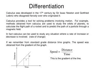
d Distance t Time Differentiation Calculus was developed in the 17th century by Sir Issac Newton and Gottfried Leibniz who disagreed fiercely over who originated it. Calculus provides a tool for solving problems involving motion. For example, methods obtained from calculus are used to study the orbits of planets, to calculate the flight path of a rocket and to predict the path of a particle through a magnetic field. In fact calculus can be used to study any situation where a rate of increase or decrease is involved. (rate of change) If we remember from standard grade distance time graphs. The speed was obtained from the gradient of the graph. This is the gradient of the line.

y x We label this gradient To determine the speed we needed two points on the graph. This gave us the average speed between these two points. But what about the speed at a certain time? The instantaneous speed. f(x+h) f(x) h For an instantaneous gradient we require ‘h’ to be zero. Let us examine this gradient as ‘h’ gets smaller and smaller. x x+h In other words, let ‘h’ approach zero.

f(x+h) f(x) h y x x+h x • The derived function represents: • The rate of change of the function • The gradient of the tangent to the graph of the function

Using the formula for f `(x) is called differentiating from first principles.

Numerous functions were derived in this way and a pattern was noticed. In general terms:

The derivative is also called the ‘rate of change’ or the ‘gradient of the tangent to the curve’. They all mean find the derived function. 1. Find the gradient of the tangent to the curve f(x) = x2 at x = 5.

2. Smoke form a factory chimney travels in t hours. Calculate the speed (rate of change) of the smoke after 4 hours. The distance travelled by the smoke is After 4 hours, t = 4. The speed of the smoke after 4 hours is ¼ km / h.

Page 92 Exercise 6E We can also derive functions with more than one term.

Derivatives of products and quotients We can also derive more complicated expressions. Before differentiating a function we have to express it as the sum of individual terms.

Now there will be times when you have a correct answer but it will not match the one shown in the back of the book. However they could well be the same. Look at our previous answer. Always check for equality when checking your answers.

h(d) 0 d 1. A designer of an artificial ski slope describes the shape of the slope by the function d is the horizontal distance in metres and h(d) is the height in metres. Calculate the gradient of the slope 4 metres horizontally from the start of the slope. The gradient of the slope 4 metres after the start of the slope is -1.

y x Instead of writing the derivative as f `(x) we can use the Leibniz notation. This is a geometric notation. The Greek letter delta Δ means ‘change’. So going back to our gradient diagram, Δy This is normally written Δx

1. Find the derivative of y = 3x4 -5x2 – 3x + 6 At t = 9,

Equations of Tangents Hence to find the equation of a tangent we need to determine: • the coordinates (a,b) of the point • the gradient, (rate of change) at that point.

Hence (9,27) is the point. Now we need the gradient at the point (9,27).

Increasing and decreasing functions This function is increasing This function is decreasing It has a positive gradient It has a negative gradient If f(x) increases as x increases then the function is increasing. If f(x) decreases as x increases then the function is decreasing.

y x Let us look at 3 points on the graph. The function is decreasing between A and B C A The function is increasing between B and C What is the function doing at B? B If we look at the tangent to the curve at point ‘B’. It will therefore have zero gradient. It has no rate of change. We see it is horizontal. A to B B B to C The derivative of a function may be used to identify the shape of its curve. zero positive negative

0 2 Let us first consider when the function is Increasing (this is a smile parabola with roots at x = 0 and x = 2) NB This is a graph of the GRADIENT not the function.

The value of (x – 1)2 must always be positive for all values of x. This means that the value of 3(x – 1)2 must always be positive which by default means that it can never be negative for all values of x. Since the gradient is never negative the function is never decreasing.

y A to B B B to C C A x zero positive negative B Stationary points Let us remind our self of what we found earlier. We saw previously that if f `(x) = 0 the function is neither increasing or decreasing. The tangent is horizontal so the point (x, f(x)) is a stationary point. Stationary points occur when f `(x) = 0. The nature of the stationary point depends on the gradient either side of it.

y y x x Minimum turning point Maximum turning point y y x x Rising point of inflexion falling point of inflexion

We will now consider the gradient either side of the stationary points to determine their nature.

+ + + - - + - + + + + 0 - 0 slope Maximum turning point at (1,5) and minimum turning point at (2,4).

We will now consider the gradient either side of the stationary points to determine their nature.

+ + + + + - + + - 0 0 slope Rising point of inflexion at (0,0) and maximum turning point at (3,27)

1. Intercepts. • Where does the curve cut the y axis? x = 0 • Where does the curve cut the x axis (roots)? y = 0 2. Stationary Points. • Where is the curve stationary? f `(x) = 0 • What are the nature of the stationary points? 3. Behaviour. • What happens for large + / - values of x? Curve sketching When sketching curves, gather as much information as possible form the list below.

- + + - - + + - + 0 0 slope Maximum turning point (0,0) and minimum turning point at (2,-4)

y x Now lest put all this information onto a set of axis. 0 3 (2,-4)

(3,18) y y 1 1 0 0 x x (-1,-2) (-2,-12) Closed Intervals In a closed interval the maximum and minimum values of a function are either at the stationary points or at the end points of the interval. Maximum value = 18 Maximum value = 0 Minimum value = -2 Minimum value = -12

y 0 x (4,48) 1 (-2,-12) Maximum value = 48 Minimum value = -12

Maximum value = 21 Minimum value = -25/27

Graph of the derived function We can sketch the graph of the derived function f `(x) by looking at the features of the graph of f(x). This is a simple strategy but does require an understanding that you are drawing the graph of f `(x) from the graph of f(x).

f(x) f `(x) x x

f(x) f `(x) x x Draw the graph of the derived function.

Differentiation