Numerical Methods for Unsteady Heat Transfer
70 likes | 429 Vues
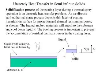
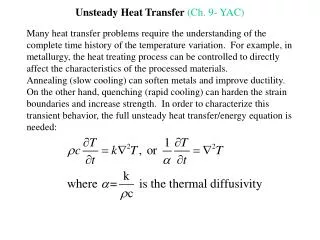
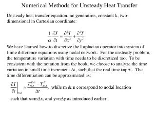
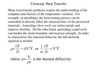
Numerical Methods for Unsteady Heat Transfer. Unsteady heat transfer equation, no generation, constant k, two-dimensional in Cartesian coordinate:.

Numerical Methods for Unsteady Heat Transfer
E N D
Presentation Transcript
Numerical Methods for Unsteady Heat Transfer Unsteady heat transfer equation, no generation, constant k, two-dimensional in Cartesian coordinate: We have learned how to discretize the Laplacian operator into system of finite difference equations using nodal network. For the unsteady problem, the temperature variation with time needs to be discretized too. To be consistent with the notation from the book, we choose to analyze the time variation in small time increment Dt, such that the real time t=pDt. The time differentiation can be approximated as:
m,n+1 Finite Difference Equations m-1,n m+1, n m,n From the nodal network to the left, the heat equation can be written in finite difference form: m,n-1
Some common nodal configurations are listed in table for your reference. On the third column of the table, there is a stability criterion for each nodal configuration. This criterion has to be satisfied for the finite difference solution to be stable. Otherwise, the solution may be diverging and never reach the final solution. For example, Fo1/4. That is, aDt/(Dx)2 1/4 and Dt(1/4a)(Dx)2. Therefore, the time increment has to be small enough in order to maintain stability of the solution. This criterion can also be interpreted as that we should require the coefficient for TPm,n in the finite difference equation be greater than or equal to zero. Question: Why this can be a problem? Can we just make time increment as small as possible to avoid it? Nodal Equations
Finite Difference Solution • Question: How do we solve the finite difference equation derived? • First, by specifying initial conditions for all points inside the nodal network. That is to specify values for all temperature at time level p=0. • Important: check stability criterion for each points. • From the explicit equation, we can determine all temperature at the next time level p+1=0+1=1. The following transient response can then be determined by marching out in time p+2, p+3, and so on.
Example Example: A flat plate at an initial temperature of 100 deg. is suddenly immersed into a cold temperature bath of 0 deg. Use the unsteady finite difference equation to determine the transient response of the temperature of the plate. L(thickness)=0.02 m, k=10 W/m.K, a=1010-6 m2/s, h=1000 W/m2.K, Ti=100C, T=0C, Dx=0.01 m Bi=(hDx)/k=1, Fo=(aDt)/(Dx)2=0.1 x 1 3 2 There are three nodal points: 1 interior and two exterior points: For node 2, it satisfies the case 1 configuration in table.