Unsteady state heat transfer
270 likes | 559 Vues
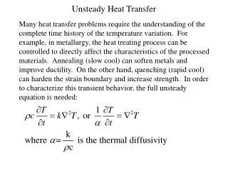
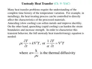
Unsteady state heat transfer . This case of heat transfer happens in different situations. It is complicated process occupies an important side in applied mathematics to find a solution for Fourier’s low as a partial differential .

Unsteady state heat transfer
E N D
Presentation Transcript
This case of heat transfer happens in different situations. • It is complicated process occupies an important side in applied mathematics to find a solution for Fourier’s low as a partial differential there are some cases unsteady heat transfer problem can be simplified to be solved using easier methods or charts prepared to give a numerical solution for some cases important in applications. -The lumped heat capacitance method. -the simplest case of unsteady heat transfer is cooling of high conductive long cylinder. Where the rate of heat transfer is :
The heat that the body loose it is transferred by conduction inside the body, this transfer from inside to outside is difficult to be calculated but it is considered that the heat transferred at once from the center to the surface as approximation. • And by this we can know temperature depression needed for the same heat transfer rate to happen. From heat transfer from center to surface and from surface to surrounding.
Where: • K:thermal conductivity [J/m.s.c] • r: radius [m] • Tc: Center temperature [C] • Ts: Surface temperature [C] • hs: convective heat transfer coefficient [J/m2.s.C] • Ta: air temperature [C].
Temperature difference between the surface and the center depends on the conductivity of the material. if the material has a high (k)the temperature difference can be neglected but (k) is low. temperature difference cannot be neglected and the following analysis can simplify that: This ratio called Biot number. If NBi<0.1, Tc=Ts L is a special dimension always used as ½ of least dimension. If Bi>0.1 means the temperature of the center of material is decreasing or increasing in slower rate than the surface and this leads to a temperature difference between the surface and center cannot be neglected.
Lumped Heat Capacitance Negligable Internal Heat Resistance • Under unsteady state heating or cooling:
x Lumped system with convective cooling Volume V y h = constant z System surface The entire volume is the system for the energy balance.
Assumption The temperature of the solid is spatially uniform at any instant during the transient process. This implies that the temperature gradients are negligible.
GRAPHICAL SOLUTIONS Heisler charts
CHARTS • This method is used in heat transfer in materials has a low conductivity coefficient. • Substitute for numerical methods. • These charts calculated from the solution for conductivity equation and drown using unit less numbers. • = temp of the cooling or heating medium • T= temp of the solid at any time t
From the charts it is possible to get results in one direction F(x), F(y), or F(z). • Or two F(x,y)= F(x).F(y) • Or three F(x,y,z)= F(x).F(y).F(z) • Charts: unsteady state heat transfer
T(0,x) = 0 h h or Bi = hL/k 2L x The infinite plate of thickness 2L
Quantities of engineering interest: (a) Temperature at x = 0as a function of time for various values of Bi = hL/k. (b) Temperature at x/L in terms of the center temperature. (c) Heat loss in terms of initial energy per unit area relative to the fluid temperature. T(0,x) = 0 h h 2L x
Mid-plane temperature, T(0,t), in a slab of thickness 2 (L=2) that is at a uniform initial temperature T0. The heat transfer coefficient, h, is the same on both surfaces. (Adapted from M. P. Heisler, 1947) Typical Heisler chart for an infinite flat plate of thickness 2L
EXAMPLES Product solutions
Product solutions. . . • How does one handle transient conduction in finite cylinder of length L and in rectangular solids? • The solutions for temperature in simple solids are expressed in terms of solutions for. . . • Infinite plates of thickness 2L • Infinite cylinders of radius R
2L1 2L3 2L2 The rectangular solid The rectangular solid is made up of the intersection of three plates of thickness 2L1, 2L2, and 2L3
The cylinder of length 2L and radius R is produced by the intersection of an infinite cylinder and an infinite plate (parallel planes). R 2L The finite length cylinder
where P(t,x) corresponds to the solution for the infinite plate, and C(t,r) to the solution for the infinite cylinder. Product solution for the cylinder
AGITATED CONTAINERS • Under unsteady state heating or cooling: Where: Tm: is the heating medium temperature. Ti: initial uniform temperature distribution of the liquid. T: is the temperature of liquid at any time
References Heisler, M. P., 1947, “Temperature Charts for Induction and Constant Temperature Heating”, Transactions, American Society of Mechanical Engineers, Vol. 69, pp. 227-236.


![Chapter 3: Unsteady State [ Transient ] Heat Conduction](https://cdn1.slideserve.com/2468294/chapter-3-unsteady-state-transient-heat-conduction-dt.jpg)