Download

1 / 27
350 likes | 1.21k Vues
Unsteady State Heat Transfer. HT3: Experimental Studies of Thermal Diffusivities and Heat Transfer Coefficients . Transient Heat Conduction. Many heat conduction problems encountered in engineering applications

E N D
Unsteady State Heat Transfer HT3: Experimental Studies of Thermal Diffusivities and Heat Transfer Coefficients
Transient Heat Conduction • Many heat conduction problems encountered in engineering applications involve time as in independent variable. The goal of analysis is to determine the variation of the temperature as a function of time and position T (x, t) within the heat conducting body. In general, we deal with conducting bodies in a three dimensional Euclidean space in a suitable set of coordinates (x ∈ R3) and the goal is to predict the evolution of the temperature field for future times (t > 0). • Here we investigate solutions to selected special cases of the following form of the heat equation Solutions to the above equation must be obtained that also satisfy suitable initial and boundary conditions.
Example: Point Thermal Explosion • Let a fixed amount of energy H0(J) be instantaneously released (thermal explosion) at time t = 0 at the origin of a three dimensional system of coordinates inside a solid body of infinite extent initially at T (X, 0) = T (r, 0) = 0 everywhere, where, . No other thermal energy input exists subsequent to the initial instantaneous release. Assuming constant thermal properties k (thermal conductivity), r (density)and Cp(heat capacity), the heat equation is: where a = k/rCp is thermal diffusivity [m2/s]. • This must be solved subject to the initial condition T (r, 0) = 0 for all r > 0 plus the statement expressing the instantaneous release of energy at t = 0 at the origin. Since the body is infinitely large, the far field temperature never changes and all the released energy must dissipate within the body itself. The fundamental solution of this problem is given by: - characteristic time where H0/rCpis the amount of energy released per unit energy required to raise the temperature of a unit volume of material by one degree. • This solution may be useful in the study of thermal explosions where a buried explosive load located at r = 0 is suddenly released at t = 0 and the subsequent distribution of temperature at various distances from the explosion is measured as a function of time. A slight modification of the solution leads to the problem of surface heating of bulk samples by short duration pulses of finely focused high energy beams.
One-Dimensional Problems • Imposed Boundary Temperature in Cartesian Coordinates: A simple but important conduction heat transfer problem consists of determining the temperature history inside a solid flat wall which is quenched from a high temperature. More specifically, consider the homogeneous problem of finding the one-dimensional temperature distribution inside a slab of thickness L and thermal diffusivity a, initially at some specified temperature T (x, 0) = f(x) and exposed to heat extraction at its boundaries x = 0 and x = L such that T (0, t) = T (L, t) = 0 (Dirichlet homogeneous conditions), for t > 0. The thermal properties are assumed constant. • Convection at the Boundary in Cartesian Coordinates: Same geometry BUT the boundary conditions specify values of the normal derivative of the temperature or when linear combinations of the normal derivative and the temperature itself are used. Consider the homogeneous problem of transient heat conduction in a slab initially at a temperature T = f(x) and subject to convection losses into a medium at T = 0 at x = 0 and x = L. Convection heat transfer coefficients at x = 0 and x = L are, respectively h1and h2. Assume the thermal conductivity of the slab k is constant. • Imposed Boundary Temperature and Convection at the Boundary in Cylindrical Coordinates: • a long cylinder (radius r = b) initially at T = f(r) whose surface temperature is made equal to zero for t > 0. • A long cylinder (radius r = b) initially at T = f(r) is exposed to a cooling medium which extracts heat uniformly from its surface. • Imposed Boundary Temperature and Convection at the Boundary in Spherical Coordinates: • quenching problem where a sphere (radius r = b) initially at T = f(r) whose surface temperature is made equal to zero for t > 0. • Consider a sphere with initial temperature T (r, 0) = f(r) and dissipating heat by convection into a medium at its surface r = b.
First Problem: Slab/Convection • The first problem is the 1D transient homogeneous heat conduction in a plate of span L from an initial temperature Ti and with one boundary insulated and the other subjected to a convective heat flux condition into a surrounding environment at T∞. This problem is equivalent to the quenching of a slab of span 2L with identical heat convection at the external boundaries x = −L and x = L). The mathematical formulation of the problem is to find T (x, t) such that: Boundary conditions: + h(T-)=0 Initial conditions: for all x when t = 0, Introduction of the following non dimensional parameters simplifies the mathematical formulation of the problem. The dimensionless distance (X), time (t) and temperature (q): and a Biot number: The Biot number (Bi) is a dimensionless number used in heat transfer calculations. It is named after the French physicistJean-Baptiste Biot (1774–1862), and gives a simple index of the ratio of the heat transfer resistances inside (1/k) of and at the surface of a body (1/hL). Biot number smaller than 0.1 imply that the heat conduction inside the body is much faster than the heat convection away from its surface, and temperature gradients are negligible inside of it.
First Problem Formulation: Slab/Convection Boundary conditions: + h(T-)=0 Initial conditions: for all x when t = 0, Introduction of the following non dimensional parameters simplifies the mathematical formulation of the problem. The dimensionless distance (X), time (t) and temperature (q) and a Biot number: With the new variables, the mathematical formulation of the heat conduction problem becomes: and
Second Problem Formulation: Solid Cylinder/Convection 1D transient homogeneous heat conduction in a solid cylinder of radius b from an initial temperature Ti and with one boundary insulated and the other subjected to a convective heat flux condition into a surrounding environment at T∞. Boundary conditions: + h(T-)=0 Introduction of the following non dimensional parameters simplifies the mathematical formulation of the problem. The dimensionless distance (X), time (t) and temperature (q) and a Biot number: With the new variables, the mathematical formulation of the heat conduction problem becomes:
Third Problem Formulation: Sphere/Convection Cooling of a sphere (0 ≤ r ≤ b) initially at a uniform temperature Ti and subjected to a uniform convective heat flux at its surface into a medium at T∞ with heat transfer coefficient h. In terms of the new variable U(r, t) = rT (r, t) the mathematical formulation of the problem is: Introduction of the following non dimensional parameters simplifies the mathematical formulation of the problem. The dimensionless distance (X), time (t) and temperature (q) and a Biot number: With the new variables, the mathematical formulation of the heat conduction problem becomes:
Fourier number • In physics and engineering, the Fourier number (Fo) or Fourier modulus, named after Joseph Fourier, is a dimensionless number that characterizes heat conduction. Conceptually, it is the ratio of diffusive/conductive transport rate by the quantity storage rate and arises from non-dimensionalization of the heat equation. The general Fourier number is defined as: Fo = Diffusive transport rate (a/L2)/storage rate (1/t) • The thermal Fourier number is defined by the conduction rate to the rate of thermal energy storage: • Compare with non-dimensionless time parameter: So Fo=t = To understand the physical significance of the Fourier number t, we may express it as Therefore, again the Fourier number is a measure of heat conducted through a body relative to heat stored. Thus, a large value of the Fourier number indicates faster propagation of heat through a body.
Lumped System Analysis if the internal temperature of a body remains relatively constant with respect to distance – can be treated as a lumped system analysis – heat transfer is a function of time only, T = T (t) Typical criteria for lumped system analysis is Bi< 0.1 • In heat transfer analysis, some bodies are observed to behave like a “lump” whose interior temperature remains essentially uniform at all times during a heat transfer process. The temperature of such bodies can be taken to be a function of time only, T(t). Heat transfer analysis that utilizes this idealization is known as lumped system analysis , which provides great simplification in certain classes of heat transfer problems without much sacrifice from accuracy. Consider a small hot copper ball coming out of an oven. Mea- surements indicate that the temperature of the copper ball changes with time, but it does not change much with position at any given time. Thus the temperature of the ball remains nearly uniform at all times, and we can talk about the temperature of the ball with no reference to a specific location.
Lumped System Analysis If Bi< 0.1 Consider a body of arbitrary shape of mass m, volume V, surface area As, density r, and specific heat cpinitially at a uniform temperature Ti. At time t =0, the body is placed into a medium at temperature T∞,and heat transfer takes place between the body and its environment, with a heat transfer coefficient h. For the sake of discussion, we assume that T>Ti, but the analysis is equally valid for the opposite case. We assume lumped system analysis to be applicable, so that the temperature remains uniform within the body at all times and changes with time only, T=T(t). During a differential time interval dt, the temperature of the body rises by a differential amount dT.An energy balance of the solid for the time interval dtcan be expressed as: =-Bi∙Fo or or Integrating from t=0, at which T =Ti, to any time t, at which T=T(t), gives The reciprocal of bhas time unit, and is called the time constant. or The temperature of a body approaches the ambient temperature T exponentially. The temperature of the body changes rapidly at the beginning, but rather slowly later on. A large value of bindicates that the body approaches the environment temperature in a short time. The larger the value of the exponent b, the higher the rate of decay in temperature. Note that b is proportional to the surface area, but inversely proportional to the mass and the specific heat of the body. This is not surprising since it takes longer to heat or cool a larger mass, especially when it has a large specific heat.
Lumped System Analysis If Bi< 0.1 (A) Once the temperature T(t) at time t is available, the rate of convection heat transfer between the body and its environment at that time can be determined from Newton’s law of cooling as: (B) The total amount of heat transfer between the body and the surrounding medium over the time interval t 0 to t is simply the change in the energy content of the body: The amount of heat transfer reaches its upper limit when the body reaches the surrounding temperature T. Therefore, the maximum heat transfer between the body and its surroundings is We could also obtain this equation by substituting the T(t) relation from Eq. A into the relation in Eq. B and integrating it from t =0 to t → ∞.
Exact Solution of One-Dimensional Transient Conduction Problem • The non-dimensionalized partial differential equation formulated above together with its boundary and • initial conditions can be solved using several analytical and numerical techniques, including the Laplace or other transform methods, the method of separation of variables, the finite difference method, and the finite-element method. • Here we discuss the method of separation of variables developed by J. Fourier in 1820s and is based on • expanding an arbitrary function (including a constant) in terms of Fourier series. The method is applied • by assuming the dependent variable to be a product of a number of functions, each being a function of a single independent variable. This reduces the partial differential equation to a system of ordinary differential equations, each being a function of a single independent variable. • In the case of transient conduction in a plain wall, for example, the dependent variable is the solution • function u(X, t), which is expressed as u(X, t)= F(X)G(t), and the application of the method results in two ordinary differential equation, one in X and the other in t. • The method is applicable if (1) the geometry is simple and finite (such as a rectangular block, a cylinder, or a • sphere) so that the boundary surfaces can be described by simple mathematical functions, and (2) the differential equation and the boundary and initial conditions in their most simplified form are linear (no terms that involve products of the dependent variable or its derivatives) and involve only one nonhomogeneous term (a term without the dependent variable or its derivatives).
Separation of Variables • Let us consider the Slab/Convection experiment. Recall that in this case we have: The heat conduction equation in cylindrical or spherical coordinates can be nondimensionalizedin a similar way. Note that nondimensionalizationreduces the number of independent variables and parameters from 8 to 3—from x, L, t, k, a, h, Ti, and T to X, Bi, and Fo. That is, This makes it very practical to conduct parametric studies and to present results in graphical form. Recall that in the case of lumped system analysis, we had u f(Bi, Fo) with no space variable.
Separation of Variables • First, we express the dimensionless temperature function u(X, t) as a product of a function of X only and a function of t only as: • Substituting to: • all the terms that depend on X are on the left-hand side of the equation and all the terms that depend on t are on the r the terms that are function of different variables are separated (and thus the name separation of variables). Considering that both X and t can be varied independently, the equality in Eq. C can hold for any value of X and t only if it is equal to a constant. Further, it must be a negative constant that we will indicate by -l2since a positive constant will cause the function G(t) to increase indefinitely with time (to be infinite), which is unphysical, and a value of zero for the constant means no time dependence, which is again inconsistent with the physical problem. Setting Eq. C equal to -l2 gives: • whose general solutions are: • and (C) we have
Separation of Variables Then it follows that there are an infinite number of solutions of the form , and the solution of this linear heat conduction problem is a linear combination of them, The constants Anare determined from the initial condition This is a Fourier series expansion that expresses a constant in terms of an infinite series of cosine functions. Now we multiply both sides of last eq. by cos(lmX), and integrate from X=0 to X=1. The right-hand side involves an infinite number of integrals of the form: It can be shown that all of these integrals vanish except when n m, and the coefficient An becomes:
Separation of Variables This completes the analysis for the solution of one-dimensional transient heat conduction problem in a plane wall. Solutions in other geometries such as a long cylinder and a sphere can be determined using the same approach. The results for all three geometries are summarized in Table. Note that the solution for the plane wall is also applicable for a plane wall of thickness L whose left surface at x =0 is insulated and the right surface at x=L is subjected to convection since this is precisely the mathematical problem we solved.
Approximate Analytical Solutions • The analytical solutions of transient conduction problems typically involve infinite series, and thus the evaluation of an infinite number of terms to determine the temperature at a specified location and time. However, as demonstrated in Table, the terms in the summation decline rapidly as n and thus lnincreases because of the exponential decay function . This is especially the case when the dimensionless time t is large. Therefore, the evaluation of the first few terms of the infinite series (in this case just the first term) is usually adequate to determine the dimensionless temperature q. For example, for t>0.2, keeping the first term and neglecting all the remaining terms in the series results in an error under 2 percent. • We are usually interested in the solution for times with t>0.2, and thus it is very convenient to express the solution using this one-term approximation, given as: where the constants A1 and l1 are functions of the Bi number only, and their values are listed in Table (see next slide) against the Bi number for all three geometries. The function J0 is the zeroth-order Bessel function of the first kind (see next slide).
Approximate Analytical Solutions • Noting that cos (0)= J0(0)= 1 and the limit of (sin x)/x is also 1, these relations simplify to the next ones at the center of a plane wall, cylinder, or sphere: • Comparing the sets of equations above with approximate solution we notice that the dimensionless temperatures anywhere in a plane wall, cylinder, and sphere are related to the center temperature by • which shows that time dependence of dimensionless temperature within a given geometry is the same throughout. That is, if the dimensionless center temperature q0drops by 20 percent at a specified time, so does the dimensionless temperature q0 anywhere else in the medium at the same time. Once the Bi number is known, these relations can be used to determine the • temperature anywhere in the medium.
Graphical Solutions : Heisler Charts The solutions obtained for 1D non homogeneous problems with Neumann boundary conditions in Cartesian coordinate systems using the method of separation of variables have been collected and assembled in the form of transient temperature nomographs by Heisler. The given charts are a very useful baseline against, which to validate one’s own analytical or numerical computations. Indeed, the determination of the constants A1and l1 usually requires interpolation. For those who prefer reading charts to interpolating, these relations are plotted and the one-term approximation solutions are presented in graphical form, known as the transient temperature charts. The transient temperature charts shown in next slides for a large plane wall, long cylinder, and sphere were presented by M. P. Heisler in 1947 and are called Heisler charts. There are three charts associated with each geometry: the first chart is to determine the temperature T0 at the center of the geometry at a given time t. The second chart is to determine the temperature at other locations at the same time in terms of T0. The third chart is to determine the total amount of heat transfer up to the time t. These plots are valid for t> 0.2.
Transient temperature and heat transfer charts for a plane wall of thickness 2L initially at a uniform temperature Tisubjected to convection from all sides to an environment at temperature T∞ with a convection coefficient of h.
Transient temperature and heat transfer charts for a long cylinder of radius roinitially at a uniform temperature Tisubjected to convection from all sides to an environment at temperature T∞ with a convection coefficient of h.
Transient temperature and heat transfer charts for a sphere of radius roinitially at a uniform temperature Tisubjected to convection from all sides to an environment at temperature T∞ with a convection coefficient of h.
Useful Relationship • Again the temperature of the body changes from the initial temperature Ti to the temperature of the surroundings T∞at the end of the transient heat conduction process and the maximum amount of heat that a body can gain (or lose) is simply the change in the energy content of the body: • The amount of heat transfer Q at a finite time t is • Assuming constant properties, the ratio of Q/Qmaxbecomes • Using the appropriate non-dimensional temperature relations based on the one term approximation for the plane wall, cylinder, and sphere, and performing the indicated integrations, we obtain the following relations for the fraction of heat transfer in those geometries: • These Q/Qmax ratio relations based on the one-term approximation are also plotted in Heisler charts, against the variables Bi and h2at/k2for the large plane wall, long cylinder, and sphere, respectively. Note that once the fraction of heat transfer Q/Qmax has been determined from these charts or equations for the given t, the actual amount of heat transfer by that time can be evaluated by multiplying this fraction by Qmax.


![Chapter 3: Unsteady State [ Transient ] Heat Conduction](https://cdn1.slideserve.com/2468294/chapter-3-unsteady-state-transient-heat-conduction-dt.jpg)