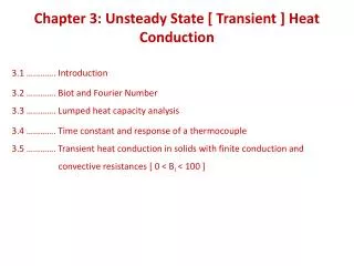
Chapter 3: Unsteady State [ Transient ] Heat Conduction

1. Chapter 3: Unsteady State [ Transient ] Heat Conduction 3.1 …………. Introduction 3.2 …………. Biot and Fourier Number 3.3 …………. Lumped heat capacity analysis 3.4 …………. Time constant and response of a thermocouple 3.5 …………. Transient heat conduction in solids with finite conduction and convective resistances [ 0 < Bi < 100 ]

2. 3.1… Introduction • Steady-state conduction: • temperature do not change with time; • equilibrium condition • unsteady-state conduction: • temperature change with time • For example, in metallurgy, the heat treating process can be controlled to directly affect the characteristics of the processed materials. Annealing (slow cool) can soften metals and improve ductility. On the other hand, quenching (rapid cool) can harden the strain boundary and increase strength. • The temperature of such a body varies with time as well as position. • T(x,y,z,t) • (x,y,z) - Variation in the x, y and z directions and t - Variation with time • Temperature will vary with location within a system and with time. NOTE: Temperature and rate heat transfer variation of a system are dependent on its internal resistance and surface resistance

3. 3.2… Biot and Fourier Number Biot Number,

4. Biot and Fourier Number (continue….) Note: Whenever the Biot number is small, the internal temperature gradients are also small and a transient problem can be treated by the “lumped thermal capacity” approach. The lumped capacity assumption implies that the object for analysis is considered to have a single mass-averaged temperature. The Fourier number (Fo) or Fourier modulus, named after Joseph Fourier, is a dimensionless number that characterizes transient behavior of a system. Conceptually, it is the ratio of the heat conduction rate to the rate of thermal energy storage. It is defined as:

5. 3.3 … Lumped heat capacity analysis The simplest situation in an unsteady heat transfer process is to use the lumped capacity analysis. Note: Neglect the temperature distribution inside the solid and only deal with the heat transfer between the solid and the ambient fluids. • Large potato put in a vessel with boiling water. • After few minutes, if you take out the potato, temperature distribution within the potato is not even close to being uniform. • Thus, lumped system analysis is not applicable in this case. • Temperature of the metal ball changes with time, but it does not change with position at any given time. • Temperature of the ball remains uniform at all times Note: The first step in the application of lumped system analysis is the calculation of the Biot number, and the assessment of the applicability of this approach. One may still wish to use lumped system analysis even when the criterion Bi ≤0.1 is not satisfied, if high accuracy is not a major concern.

6. 3.4 … Time constant and response of a thermocouple Thermocouple: When two dissimilar metals are joined together at two points to form a closed loop and temperature difference exists between junctions, an electrical potential is set up between the junctions. Such an arrangement is known as thermocouple and is frequently used for the temperature measurement and used in lumped parameter analysis. Response of a thermocouple: Time required for the thermocouple to reach the source temperature when it is exposed to it. Sensitivity: Time required by the thermocouple to reach 63.2% of its steady state value.

7. Time constant and response of a thermocouple(continue….) The parameter ρVc/hA has units of time and is called time constant of the system and denoted by τ *. Using time constant, the temperature distribution in the solid can be expressed as Note: Low value of time constant can be achieved by (i) decreasing the wire diameter (ii) using light metals of low density and low specific heat (iii) increasing the heat transfer coefficient

8. 3.5 … Transient heat conduction in solids with finite conduction and convective resistances [ 0 < Bi < 100 ] • Consider the heating and cooling of a plane wall of thickness l = 2δ and extending to infinity in the y and z direction. Initially the wall is at uniform temperature ti and suddenly both surfaces +δ and – δ are exposed to and maintained at the ambient temperature ta. The controlling equation for the transient heat conduction is: • Boundary conditions are: • t = ti at τ=0 • dt/dx=0 at x=0; symmetric nature of the • temperature profile within the plane wall; • Conduction = convection • kA(dt/dx)=hA(t-ta) at x= + δ and x= – δ • The solution obtained after mathematical analysis that

9. Obvious when conduction resistance is not negligible, the temperature history becomes a function of Biot number hl/k, Fourier number ατ/l2 and the dimensionless parameter x/l which indicates the location of point within the plate where temperature is to be obtained. Note: In case of cylinder and sphere x/l is replaced by r/R. Graphical charts have been prepared for the above equation in a variety of forms. The Hiesler charts depict the dimensionless temperature (to-ta)/(ti-ta) versus Fo for various values of 1/Bi for solids of different geometrical shapes such as a plate, cylinders and spheres. Note: Hiesler charts give the temperature history of the solid at its mid plane, x=0. Temperatures at other locations are worked out by multiplying the mid plane temperature by the correction factors read from charts which is given. Use is made of the following relationship.