STEADY-STATE, MULTI-DIMENSIONAL CONDUCTION
STEADY-STATE, MULTI-DIMENSIONAL CONDUCTION. Analytical Method: Separation of Variables Conduction Factor and Dimensionless Conduction Heat Rate Numerical Method: Finite Difference Method Finite Volume Method.

STEADY-STATE, MULTI-DIMENSIONAL CONDUCTION
E N D
Presentation Transcript
STEADY-STATE, MULTI-DIMENSIONAL CONDUCTION • Analytical Method: • Separation of Variables • Conduction Factor and Dimensionless Conduction Heat Rate • Numerical Method: • Finite Difference Method • Finite Volume Method
Eigenvalue problem in the direction of homogeneous boundary condition Analytical Method Separation of Variables + Boundary conditions 1) Equation : linear and homogeneous 2) Boundary condition : homogeneous at least in one direction
over or boundary conditions : Sturm-Liouville Theory Sturm-Liouville System : Hermitian operator (self-adjoint operator) w(x) : weighting function Corresponding eigenvalue problem
boundary terms = boundary terms thus Definition of inner product : formally self-adjoint operator
i) ii) when or and can be finite. iii) when either at a or b boundary terms homogeneous boundary conditions
When Ex) self-adjoint operator
: at least piecewise continuous function : eigenfunction Properties of Hermitian operator • eigenvalues : all real • eigenfunctions : orthogonal • eigenfunctions : a complete set orthogonality: : least square convergence
Example : Laplace equation y x assume then Ex) 1) in (x,y) coordinate system (Cartesian) with homogeneous boundary conditions in the x direction This is a special case of S-L system with eigenfunctions : trigonometric functions, sinx or cosx
r z assume , then or or This is a special case of S-L system with Remark : transform with Bessel equation : Ex) 2) in (r,z) coordinate system (cylindrical) with homogeneous boundary conditions in the r direction eigenfunctions : Bessel functions
r q with homogeneous boundary conditions in the q direction assume equation for or with or This is a special case of S-L system with Legendre equation : Remark 3) in (r,q) coordinate system (spherical) eigenfunctions : Legendre functions
T2 T1 T1 T1 Let Two dimensional conduction in a thin rectangular plate or a long rectangular rod with no heat generation y W T(x,y) b.c. x 0 L b.c.
y 1 Let W 0 q(x,y) 0 x 0 L 0 or Dividing both sides by XY, = constant
y 1 W 0 q(x,y) 0 x 0 L 0 boundary conditions
For X(x): b.c. To be non-trivial : eigenvalue : eigenfunction
For Y(y): b.c. particular solution:
Multiply both sides by and integrate fromx = 0 toL
Solution: where
Td 0 0 0 Td Ta Tb Ta 0 0 Tb 0 0 0 = + + + 0 0 0 Tc 0 Tc -T3(x) T0 T0 T0 0 adiabat 0 0 0 0 0 = 0 0 0 0 = 0 0 + 0 + + T1 0 0 0 adiabat 0 0 0 0 -T3(x) Method of Superposition 1) inhomogeneous boundary condition T = T1 + T2 + T3 + T4 2) inhomogeneous equation T = T1 + T2 = T1+ T3 + T4
T(ro,z) = 0 T(r,l) = Tl T(r,0) = 0 or Cylindrical Rod r z ro l boundary conditions r: finite, z:
T(ro,z) = 0 r T(r,l) = Tl T(r,0) = 0 z ro l = finite Boundary conditions = finite
= finite, Let then or thus as = finite: such that For R(r): b.c.
eigenfunction: l1ro l2ro l3ro l4ro
For Z(z): b.c.
Solution: where
Conduction Shape Factor and Dimensionless Heat Transfer Rate Conduction Shape Factor S: shape factor S : determined analytically two-dimensional conduction resistance
A T1 T2 L T2 T1 Ex) Plane wall Cylindrical wall
Conduction shape factors and dimensionless conduction heat rates for selected systems
or Dimensionless Heat Transfer Rate Objects at isothermal temperature (T1) embedded with an infinite medium of uniform temperature (T2) Characteristic length Dimensionless conduction heat rate
(m,n+1) cell (m-1,n) (m+1,n) (m,n) Dy (m,n-1) Dx Numerical Method Finite Difference Method grid discretization node (nodal point)
or Similarly,
If we neglect (truncation error) and when
(m,n+1) (m-1,n) (m+1,n) (m,n) Dy (m,n-1) Dx Finite Volume Method (Energy Balance Method) Assumption of linear temperature profile
Then, Similarly, If
Convection Boundary Conditions 1) Side (m,n+1) h, T∞ (m,n) (m-1,n) Dy (m,n-1) Dx If or
2) Corner (m,n) (m-1,n) (m,n-1) Dy Dx If
3) Internal corner (m,n+1) (m-1,n) (m,n) (m+1,n) Dy (m,n-1) Dx If or
1) Analytical method (matrix inversion) → Cramer’s rule Ifn = 10, 3×10⁶operations. Ifn = 25, IBM360 1017years 2) Direct (elimination) method (n < 40) Gauss-Jordan elimination method Augmented matrix of operations
3) Gauss-Seidel iteration method (n > 100) diagonal dominance → sufficient condition for convergence convergence criterion
Dx = 0.25 m Dy = 0.25 m 1 2 1 3 4 3 5 6 5 7 8 7 Example 4.3 Ts = 500 K Fire clay brick 1 m ×1 m k = 1 W/m.K Ts = 500 K Ts = 500 K Find: Temperature distribution and heat rate per unit length T∞ = 300 K h = 10 W/m2.K Air Nodes at the plane surface with convection: When Dx = Dy,
inner nodes: convection nodes: Node 1: Node 3: Node 5: Node 2: Node 4: Node 6: Node 7: Node 8: Ts = 500 K 1 2 1 3 4 3 Ts = 500 K Ts = 500 K 5 6 5 7 8 7 T∞ = 300 K h = 10 W/m2.K
Using a standard matrix inversion routine, it is a simple matter to find the inverse of , giving