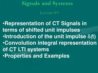
Signals and Systems Lecture 4
300 likes | 536 Vues
Signals and Systems Lecture 4. Representation of signals Convolution Examples. Chapter 2 LTI Systems. 1. 1. L. L. 0 2 t. 0 1 2 t. 1. 1.

Signals and Systems Lecture 4
E N D
Presentation Transcript
Signals and SystemsLecture 4 Representation of signals Convolution Examples
Chapter 2 LTI Systems 1 1 L L 0 2 t 0 1 2 t 1 1 0 2 4 t 0 2 4 t -1 Example 1 an LTI system
Chapter 2 LTI Systems n §2.1 Discrete-time LTI Systems : The Convolution Sum (卷积和) §2.1.1 The Representation of Discrete-Time Signals in Terms of impulses Example 2
Representing DT Signals with Sums of Unit Samples • Property of Unit Sample • Examples
Written Analytically Coefficients Basic Signals Important to note the “-” sign Note the Sifting Property of the Unit Sample
Chapter 2 LTI Systems §2.1.2 The Discrete-Time Unit Impulse Responses and the Convolution-Sum Representation of LTI Systems • The Unit Impulse Responses • 单位冲激响应 2. Convolution-Sum (卷积和) k时刻的脉冲在n时刻的响应 系统在n时刻的输出包含所有时刻输入脉冲的影响
Derivation of Superposition Sum • Now suppose the system is LTI, and define the unit sample response h[n]: • From Time-Invariance: • From Linearity: convolution sum
The Superposition Sum for DT Systems Graphic View of Superposition Sum
Hence a Very Important Property of LTI Systems • The output of any DT LTI System is a convolution of the input signal with the unit-sample response, i.e. • As a result, any DT LTI Systems are completely characterizedby its unit sample response
Calculation of Convolution Sum • Choose the value of n and consider it fixed View as functions of k with n fixed From x[n] and h[n] to x[k] and h[n-k] Note, h[n-k]–k is the mirror image of h[n]–n with the origin shifted to n
Calculating Successive Values: Shift, Multiply, Sum • y[n] = 0 for n < • y[-1] = • y[0] = • y[1] = • y[2] = • y[3] = • y[4] = • y[n] = 0 for n > -1 1 2 -2 -3 1 1 4
Calculation of Convolution SumUse of Analytical Form • Suppose that and then
Calculation of Convolution SumExample of Array Method • If x[n]<0 for n<-1,x[-1]=1,x[0]=2,x[1]=3, x[4]=5,…,and h[n]<0 for n<-2,h[-2]=-1, h[-1]=5,h[0]=3,h[1]=-2,h[2]=1,….In this case ,N=-1,M=-2,and the array is as follows So,y[-3]=-1, y[-2]=3, y[-1]=10, y[0]=15, y[1]=21,…, and y[n]=0 for n<-3
Calculation of Convolution SumUsing Matlab • The convolution of two discrete-time signals can be carried out using the Matlab M-file conv. • Example: • p=[0 ones(1,10) zeros(1,5)]; • x=p; h=p; • y=conv(x,h); • n=-1:14; • subplot(2,1,1),Stem(n, x(1:length(n))) • n=-2:24; • subplot(2,1,2),Stem(n, y(1:length(n)))
Conclusion • Any DT LTI Systems are completely characterizedby its unit sample response. • Calculation of convolution sum: • Step1:plot x and h vs k, since the convolution sum is on k; • Step2:Flip h[k] around vertical axis to obtain h[-k]; • Step3:Shift h[-k] by n to obtain h[n-k] ; • Step4:Multiply to obtain x[k]h[n-k]; • Step5:Sum on k to compute • Step6:Index n and repeat step 3 to 6.
Conclusion • Calculation Methods of Convolution Sum • Using graphical representations; • Compute analytically; • Using an array; • Using Matlab.
Chapter 2 LTI Systems §2.2 Continuous-Time LTI Systems : The Convolution Integral (卷积积分) §2.2.1 The Representation of Continuous-Time Signals in Terms of impulses ——Sifting Property §2.2.2 The Continuous-Time Unit Impulse Response and the Convolution Integral Representation of LTI Systems
Representation of CT Signals • Approximate any input x(t) as a sum of shifted, scaled pulses (in fact, that is how we do integration)
Representation of CT Signals (cont.) ⇓ Sifting property of the unit impulse ↓ limit as Δ → 0
Response of a CT LTI System • Now suppose the system is LTI, and define the unit impulse response h(t): δ(t) → h(t) • From Time-Invariance: δ(t − τ) → h(t − τ) • From Linearity:
Superposition Integral for CT Systems Graphic View of Staircase Approximation
CT Convolution Mechanics • To compute superposition integral • Step1:plot x and h vs τ, since the convolution integral is on τ; • Step2:Flip h(τ) around vertical axis to obtain h(-τ); • Step3:Shift h(-τ) by n to obtain h(n-τ) ; • Step4:Multiply to obtain x(τ)h(n-τ); • Step5:Integral on τ to compute • Step6:Increase t and repeat step 3 to 6.
Basic Properties of Convolution • Commutativity: x(t)∗ h(t) = h(t) ∗ x(t) • Distributivity: • Associativity: • x(t)∗ δ(t − to ) = x(t − to ) (Sifting property: x(t) ∗ δ(t) = x(t)) • An integrator:
More about Response of LTI Systems • How to get h(t) or h[n]: • By experiment; • May be computable from some known mathematical representation of the given system. • Step response:
Summary • What we have learned ? • The representation of DT and CT signals; • Convolution sum and convolution integral Definition; Mechanics; • Basic properties of convolution; • What was the most important point in the lecture? • What was the muddiest point? • What would you like to hear more about?
Readlist • Signals and Systems: • 2.3,2.4 • P103~126 • Question: The solution of LCCDE (Linear Constant Coefficient Differential or Difference Equations)
Problem Set • 2.21(a),(c),(d) • 2.22(a),(b),(c)
