Vector Field Topology
Vector Field Topology. Josh Levine 4-11-05. Overview. Vector fields (VFs) typically used to encode many different data sets: e.g. Velocity/Flow, E&M, Temp., Stress/Strain Area of interest: Visualization of VFs Problem: Data overload!

Vector Field Topology
E N D
Presentation Transcript
Vector Field Topology Josh Levine 4-11-05
Overview • Vector fields (VFs) typically used to encode many different data sets: • e.g. Velocity/Flow, E&M, Temp., Stress/Strain • Area of interest: Visualization of VFs • Problem: Data overload! • One solution: Visualize a “skeleton” of the VF by viewing its topology
Vector Fields • A steady vector field (VF) is defined as a mapping: • v: N → TN, N a manfold, TN the tang. bundle of N • In general, N = TN ≈ Rn • An integral curve is defined by a diff. eqn: • df/dt = v(f(t)), with fo, to as initial conditions • Also called streamlines
Vector Fields • A phase portrait is a depiction of these integral curves: Image: A Combinatorial Introduction to Topology, Michael Henle
Critical Points • A critical point is a singularity in the field such that v(x) = 0. • Critical points are classified by eigenvalues of the Jacobian matrix, J, of the VF at their position: • e.g. in 2d, • If J has full rank, the critical point is called linear or first-order • Hyperbolic critical points have nonzero real parts
Critical Points Image: Surface representations of 2- and 3-dimensional fluid flow topology, Helman & Hesselink
Critical Points • Generally: • R > 0 refers to repulsion • R < 0 refers to attraction • e.g. a saddle both repels and attracts • I ≠ 0 refers to rotation • e.g. a focus and a center • Note in 2d case I1 = -I2
Sectors & Separatrices • In the vicinity of a critical point, there are various sectors or regions of different flow type: • hyperbolic: paths do not ever reach c.p. • parabolic: one end of all paths is at c.p. • elliptic: all paths begin & end at c.p. • A separatrix is the bounding curve (or surface) which separates these regions
Sectors & Separatrices Images: A topology simplification method for 2D vector fields. Xavier Tricoche, Gerik Scheuermann, & Hans Hagen
Sectors & Separatrices Images: A topology simplification method for 2D vector fields. Xavier Tricoche, Gerik Scheuermann, & Hans Hagen
Planar Topology • Planar topology of a VF is simply a graph with the critical points as nodes and the separatrices as edges. e.g.:
Poincaré Index • Another topological invariant • The index (a.k.a. winding number) of a critical point is number of VF revolutions along a closed curve around that critical point • By continuity, always an integer • The index of a closed curve around multiple critical points will be the sum of the indices of the critical points
Poincaré Index • The index around no critical point will always be zero • For first order critical points, saddle will be -1 and all others will be +1 • There is a combinatorial theory that shows:
Three Dimensions • In 3D, we classify critical points in a similar manner using the 3 eigenvalues of the Jacobian • Broadly, there are 2 cases: • Three real eigenvalues • Two complex conjugates & one real
Three Dimensions Left-to-right: Nodes, Node-Saddles, Focus, Focus-Saddles Top: Repelling variants; Bottom: Attracting variables Left-half: 3 real eigenvalues; Right-half: 2 complex eigenvalues Images: Saddle Connectors – An approach to visualizing the topological skeleton of complex 3D vector fields, Theisel, Weinkauf, Hege, and Seidel
Three Dimensions • Separatrices now become 2d surfaces and 1d curves. • Thus topology of first-order critical points will be composed of the critical points themselves + curves + surfaces Images: Saddle Connectors – An approach to visualizing the topological skeleton of complex 3D vector fields, Theisel, Weinkauf, Hege, and Seidel
Vector Field Equivalence • We can call two VFs equivalent by showing a diffeomorphism which maps integral curves from the first to the second and preserves orientation • A VF is structural stable if any perturbation to that VF results in one which is structurally equivalent • In particular, nonhyperbolic critical points (such as centers) mean a VF is unstable because an arbitrarily small perturbation can change the critical point to a hyperbolic one.
Bifurcations • Consider an unsteady (time-varying) VF: • v: N ´ I → TN, I ÍR • As time progresses, topological transitions, or bifurcations, will occur as critical points are created, merged, or destroyed • Two main classifications, local (affecting the nature of a singular point) and global (not restricted to a particular neighborhood)
Local Bifurcations • Hopf Bifurcation • A sink is transformed into a source • Creates a closed orbit around the sink: Image: Topology tracking for the visualization of time-dependent two-dimensional flows, Xavier Tricoche, Thomas Wischgol, Gerik Scheuermann, & Hans Hagen
Local Bifurcations • Also, Fold Bifurcations: • Pairwise annihilation of saddle & source/sink: Image: Topology tracking for the visualization of time-dependent two-dimensional flows, Xavier Tricoche, Thomas Wischgol, Gerik Scheuermann, & Hans Hagen
Global Bifurcations • Basin Bifurcation • Separatrices between two saddles “swap” • Creates a heteroclinic connection Image: Topology tracking for the visualization of time-dependent two-dimensional flows, Xavier Tricoche, Thomas Wischgol, Gerik Scheuermann, & Hans Hagen
Global Bifurcations • Periodic Blue Sky Bifurcation • Between a saddle and a focus • Creates a closed orbit and a source • Passes through a homoclinic connection Image: Topology tracking for the visualization of time-dependent two-dimensional flows, Xavier Tricoche, Thomas Wischgol, Gerik Scheuermann, & Hans Hagen
Visualization Images: Stream line and path line oriented topology for 2D time-dependent vector fields, Theisel, Weinkauf, Hege, and Seidel
Conclusions • By observing the topology of a VF, we present a “skeleton” of the information, i.e. the defining structure of the VF • In doing so, we can consider only areas of interest such as critical points or in the unsteady case bifurcations