V20 Extreme Pathways
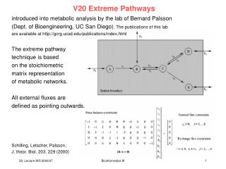
V20 Extreme Pathways. introduced into metabolic analysis by the lab of Bernard Palsson (Dept. of Bioengineering, UC San Diego) . The publications of this lab are available at http://gcrg.ucsd.edu/publications/index.html The extreme pathway technique is based on the stoichiometric

V20 Extreme Pathways
E N D
Presentation Transcript
V20 Extreme Pathways introduced into metabolic analysis by the lab of Bernard Palsson (Dept. of Bioengineering, UC San Diego). The publications of this lab are available at http://gcrg.ucsd.edu/publications/index.html The extreme pathway technique is based on the stoichiometric matrix representation of metabolic networks. All external fluxes are defined as pointing outwards. Schilling, Letscher, Palsson, J. theor. Biol. 203, 229 (2000) Bioinformatics III
Feasible solution set for a metabolic reaction network (A) The steady-state operation of the metabolic network is restricted to the region within a cone, defined as the feasible set. The feasible set contains all flux vectors that satisfy the physicochemical constrains. Thus, the feasible set defines the capabilities of the metabolic network. All feasible metabolic flux distributions lie within the feasible set, and (B) in the limiting case, where all constraints on the metabolic network are known, such as the enzyme kinetics and gene regulation, the feasible set may be reduced to a single point. This single point must lie within the feasible set. Edwards & Palsson PNAS 97, 5528 (2000) Bioinformatics III
Extreme Pathways – theorem Theorem. A convex flux cone has a set of systemically independent generating vectors. Furthermore, these generating vectors (extremal rays) are unique up to a multiplication by a positive scalar. These generating vectors will be called „extreme pathways“. (1) The existence of a systemically independent generating set for a cone is provided by an algorithm to construct extreme pathways (see below). (2) uniqueness? Let {p1, ..., pk} be a systemically independent generating set for a cone. Then follows that if pj = c´+ c´´ both c´and c´´ are positive multiples of pj. Schilling, Letscher, Palsson, J. theor. Biol. 203, 229 (2000) Bioinformatics III
Extreme Pathways – uniqueness To show that this is true, write the two pathways c´and c´´ as non-negative linear combinations of the extreme pathways: Since the pi are systemically independent, Therefore both c´and c´´ are multiples of pj. If {c1, ..., ck} was another set of extreme pathways, this argument would show that each of the ci must be a positive multiple of one of the pi. Schilling, Letscher, Palsson, J. theor. Biol. 203, 229 (2000) Bioinformatics III
Extreme Pathways – algorithm - setup The algorithm to determine the set of extreme pathways for a reaction network follows the pinciples of algorithms for finding the extremal rays/ generating vectors of convex polyhedral cones. Combine n n identity matrix (I) with the transpose of the stoichiometric matrix ST. I serves for bookkeeping. Schilling, Letscher, Palsson, J. theor. Biol. 203, 229 (2000) S I ST Bioinformatics III
separate internal and external fluxes Examine constraints on each of the exchange fluxes as given by j bj j If the exchange flux is constrained to be positive do nothing. If the exchange flux is constrained to be negative multiply the corresponding row of the initial matrix by -1. If the exchange flux is unconstrained move the entire row to a temporary matrix T(E). This completes the first tableau T(0). T(0) and T(E) for the example reaction system are shown on the previous slide. Each element of this matrices will be designated Tij. Starting with x = 1 and T(0) = T(x-1) the next tableau is generated in the following way: Schilling, Letscher, Palsson, J. theor. Biol. 203, 229 (2000) Bioinformatics III
idea of algorithm (1) Identify all metabolites that do not have an unconstrained exchange flux associated with them. The total number of such metabolites is denoted by . For the example, this is only the case for metabolite C ( = 1). What is the main idea? - We want to find balanced extreme pathways that don‘t change the concentrations of metabolites when flux flows through (input fluxes are channelled to products not to accumulation of intermediates). - The stochiometrix matrix describes the coupling of each reaction to the concentration of metabolites X. - Now we need to balance combinations of reactions that leave concentrations unchanged. Pathways applied to metabolites should not change their concentrations the matrix entries need to be brought to 0. Schilling, Letscher, Palsson, J. theor. Biol. 203, 229 (2000) Bioinformatics III
keep pathways that do not change concentrations of internal metabolites (2) Begin forming the new matrix T(x) by copying all rows from T(x – 1) which contain a zero in the column of ST that corresponds to the first metabolite identified in step 1, denoted by index c. (Here 3rd column of ST.) Schilling, Letscher, Palsson, J. theor. Biol. 203, 229 (2000) T(0) = T(1) = + Bioinformatics III
balance combinations of other pathways (3) Of the remaining rows in T(x-1) add together all possible combinations of rows which contain values of the opposite sign in column c, such that the addition produces a zero in this column. Schilling, et al. JTB 203, 229 T(0) = T(1) = Bioinformatics III
remove “non-orthogonal” pathways (4) For all of the rows added to T(x) in steps 2 and 3 check to make sure that no row exists that is a non-negative combination of any other sets of rows in T(x) . One method used is as follows: let A(i) = set of column indices j for with the elements of row i = 0. For the example above Then check to determine if there exists A(1) = {2,3,4,5,6,9,10,11} another row (h) for which A(i) is a A(2) = {1,4,5,6,7,8,9,10,11} subset of A(h). A(3) = {1,3,5,6,7,9,11} A(4) = {1,3,4,5,7,9,10} If A(i) A(h),i h A(5) = {1,2,3,6,7,8,9,10,11} where A(6) = {1,2,3,4,7,8,9} A(i) = { j : Ti,j = 0, 1 j (n+m) } then row i must be eliminated from T(x) Schilling et al. JTB 203, 229 Bioinformatics III
repeat steps for all internal metabolites (5) With the formation of T(x) complete steps 2 – 4 for all of the metabolites that do not have an unconstrained exchange flux operating on the metabolite, incrementing x by one up to . The final tableau will be T(). Note that the number of rows in T () will be equal to k, the number of extreme pathways. Schilling et al. JTB 203, 229 Bioinformatics III
balance external fluxes (6) Next we append T(E) to the bottom of T(). (In the example here = 1.) This results in the following tableau: Schilling et al. JTB 203, 229 T(1/E) = Bioinformatics III
balance external fluxes (7) Starting in the n+1 column (or the first non-zero column on the right side), if Ti,(n+1) 0 then add the corresponding non-zero row from T(E) to row i so as to produce 0 in the n+1-th column. This is done by simply multiplying the corresponding row in T(E) by Ti,(n+1) and adding this row to row i . Repeat this procedure for each of the rows in the upper portion of the tableau so as to create zeros in the entire upper portion of the (n+1) column. When finished, remove the row in T(E) corresponding to the exchange flux for the metabolite just balanced. Schilling et al. JTB 203, 229 Bioinformatics III
balance external fluxes (8) Follow the same procedure as in step (7) for each of the columns on the right side of the tableau containing non-zero entries. (In this example we need to perform step (7) for every column except the middle column of the right side which correponds to metabolite C.) The final tableau T(final) will contain the transpose of the matrix P containing the extreme pathways in place of the original identity matrix. Schilling et al. JTB 203, 229 Bioinformatics III
pathway matrix T(final) = PT = Schilling et al. JTB 203, 229 v1 v2 v3 v4 v5 v6 b1 b2 b3 b4 p1 p7 p3 p2 p4 p6 p5 Bioinformatics III
Extreme Pathways for model system 2 pathways p6 and p7 are not shown (right below) because all exchange fluxes with the exterior are 0. Such pathways have no net overall effect on the functional capabilities of the network. They belong to the cycling of reactions v4/v5 and v2/v3. Schilling et al. JTB 203, 229 v1 v2 v3 v4 v5 v6 b1 b2 b3 b4 p1 p7 p3 p2 p4 p6 p5 Bioinformatics III
How reactions appear in pathway matrix In the matrix P of extreme pathways, each column is an EP and each row corresponds to a reaction in the network. The numerical value of the i,j-th element corresponds to the relative flux level through the i-th reaction in the j-th EP. Papin, Price, Palsson, Genome Res. 12, 1889 (2002) Bioinformatics III
Properties of pathway matrix A symmetric Pathway Length Matrix PLM can be calculated: where the values along the diagonal correspond to the length of the EPs. The off-diagonal terms of PLM are the number of reactions that a pair of extreme pathways have in common. Papin, Price, Palsson, Genome Res. 12, 1889 (2002) Bioinformatics III
Properties of pathway matrix One can also compute a reaction participation matrix PPM from P: where the diagonal correspond to the number of pathways in which the given reaction participates. Papin, Price, Palsson, Genome Res. 12, 1889 (2002) Bioinformatics III
EP Analysis of H. pylori and H. influenza Amino acid synthesis in Heliobacter pylori vs. Heliobacter influenza studied by EP analysis. Papin, Price, Palsson, Genome Res. 12, 1889 (2002) Bioinformatics III
Extreme Pathway Analysis Calculation of EPs for increasingly large networks is computationally intensive and results in the generation of large data sets. Even for integrated genome-scale models for microbes under simple conditions, EP analysis can generate thousands of vectors! Interpretation: - the metabolic network of H. influenza has an order of magnitude larger degree of pathway redundancy than the metabolic network of H. pylori Found elsewhere: the number of reactions that participate in EPs that produce a particular product is poorly correlated to the product yield and the molecular complexity of the product. Possible way out? Papin, Price, Palsson, Genome Res. 12, 1889 (2002) Bioinformatics III
Linear Matrices Transpose of a linear matrix A: U is a unitary n n matrix with the n n identity matrix In. In linear algebra singular value decomposition (SVD) is an important factorization of a rectangular real or complex matrix, with several applications in signal processing and statistics. This matrix decomposition is analogous to the diagonalization of symmetric or Hermitian square matrices using a basis of eigenvectors given by the spectral theorem. Bioinformatics III
Diagonalisation of pathway matrix? Suppose M is an m n matrix with real or complex entries. Then there exists a factorization of the form M = U V* where U : m m unitary matrix, Σ : is an mn matrix with nonnegative numbers on the diagonal and zeros off the diagonal, V* : the transpose of V, an n n unitary matrix of real or complex numbers. Such a factorization is called a singular-value decomposition of M. U describes the rows of M with respect to the base vectors associated with the singular values. V describes the columns of M with respect to the base vectors associated with the singular values. Σ contains the singular values One commonly insists that the values Σi,i be ordered in non-increasing fashion. In this case, the diagonal matrix Σ is uniquely determined by M (though the matrices U and V are not). Bioinformatics III
Single Value Decomposition of EP matrices For a given EP matrix P np, SVD decomposes Pinto 3 matrices where U nn : orthonormal matrix of the left singular vectors, Vpp : an analogous orthonormal matrix of the right singular vectors, rr :a diagonal matrix containing the singular values i=1..rarranged in descending order where r is the rank of P. The first r columns of U and V, referred to as the left and right singular vectors, or modes, are unique and form the orthonormal basis for the column space and row space of P. The singular values are the square roots of the eigenvalues of PTP. The magnitude of the singular values in indicate the relative contribution of the singular vectors in U and V in reconstructing P. E.g. the second singular value contributes less to the construction of P than the first singular value etc. Price et al. Biophys J 84, 794 (2003) Bioinformatics III
Single Value Decomposition of EP: Interpretation The first mode (as the other modes) corresponds to a valid biochemical pathway through the network. The first mode will point into the portions of the cone with highest density of EPs. Price et al. Biophys J 84, 794 (2003) Bioinformatics III
SVD applied for Heliobacter systems Cumulative fractional contributions for the singular value decomposition of the EP matrices of H. influenza and H. pylori. This plot represents the contribution of the first n modes to the overall description of the system. Price et al. Biophys J 84, 794 (2003) Bioinformatics III