ENE 325 Electromagnetic Fields and Waves

1. ENE 325Electromagnetic Fields and Waves Lecture 1 Electrostatics

2. Syllabus • Dr. RardchawadeeSilapunt, rardchawadee.sil@kmutt.ac.th • Lecture: 9:30pm-12:20pm Wednesday, Rm. CB41004 • Office hours :By appointment • Textbook: Fundamentals of Electromagnetics with Engineering Applications by Stuart M. Wentworth (Wiley, 2005)

3. Course Objectives • This is the course on beginning level electrodynamics. The • purpose of the course is to provide junior electrical engineering • students with the fundamental methods to analyze and • understand electromagnetic field problems that arise in various • branches of engineering science.

4. Prerequisite knowledge and/or skills • Basic physics background relevant to electromagnetism: charge, force, SI system of units; basic differential and integral vector calculus • Concurrent study of introductory lumped circuit analysis

5. Course outline Introduction to course: • Review of vector operations • Orthogonal coordinate systems and change of coordinates • Integrals containing vector functions • Gradient of a scalar field and divergence of a vector field

6. Electrostatics: • Fundamental postulates of electrostatics and Coulomb's Law • Electric field due to a system of discrete charges • Electric field due to a continuous distribution of charge • Gauss' Law and applications • Electric Potential • Conductors in static electric field • Dielectrics in static electric fields • Electric Flux Density, dielectric constant • Boundary Conditions • Capacitor and Capacitance • Nature of Current and Current Density

7. Electrostatics: • Resistance of a Conductor • Joule’s Law • Boundary Conditions for the current density • The Electromotive Force • The Biot-Savart Law

8. Magnetostatics: • Ampere’s Force Law • Magnetic Torque • Magnetic Flux and Gauss’s Law for Magnetic Fields • Magnetic Vector Potential • Magnetic Field Intensity and Ampere’s Circuital Law • Magnetic Material • Boundary Conditions for Magnetic Fields • Energy in a Magnetic Field • Magnetic Circuits • Inductance

9. Dynamic Fields: • Faraday's Law and induced emf • Transformers • Displacement Current • Time-dependent Maxwell's equations and electromagnetic wave equations • Time-harmonic wave problems, uniform plane waves in lossless media, Poynting's vector and theorem • Uniform plane waves in lossy media • Uniform plane wave transmission and reflection on normal and oblique incidence

10. Grading • Homework 20% Midterm exam 40% Final exam 40% Vision: Providing opportunities for intellectual growth in the context of an engineering discipline for the attainment of professional competence, and for the development of a sense of the social context of technology.

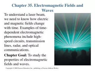
11. Examples of Electromagnetic fields • Electromagnetic fields • Solar radiation • Lightning • Radio communication • Microwave oven • Light consists of electric and magnetic fields. An electromagnetic wave can propagate in a vacuum with a speed velocity c=2.998x108m/s c = f f = frequency (Hz)  = wavelength (m)

12. Vectors - Magnitude and direction 1. Cartesian coordinate system (x-, y-, z-)

13. Vectors - Magnitude and direction 2. Cylindrical coordinate system (, , z)

14. Vectors - Magnitude and direction 3. Spherical coordinate system (, , )

15. Manipulation of vectors • To find a vector from point m to n • Vector addition and subtraction • Vector multiplication • vector  vector = vector • vector  scalar = vector

16. Ex1: Point P (0, 1, 0), Point R (2, 2, 0) • The magnitude of the vector line from the origin (0, 0, 0) to point P • The unit vector pointed in the direction of vector

17. Ex2: P (0,-4, 0), Q (0,0,5), R (1,8,0), and S (7,0,2) • a) Find the vector from point P to point Q • b) Find the vector from point R to point S

18. c) Find the direction of

19. Coulomb’s law • Law of attraction: positive charge attracts negative charge • Same polarity charges repel one another • Forces between two charges Coulomb’s Law Q=electric charge (coulomb, C)0 = 8.854x10-12 F/m 

20. Electric field intensity • An electric field from Q1 is exerted by a force between Q1 and Q2 and the magnitude of Q2 • or we can write

21. Electric field lines

22. Spherical coordinate system • orthogonal point (r,, ) • r = a radial distance from the origin to the point (m) •  = the angle measured from the positive axis (0 ) •  = an azimuthal angle, measured from x-axis (0  2) A vector representation in the spherical coordinate system:

23. Point conversion between cartesian and spherical coordinate systems

24. Unit vector conversion (Spherical coordinates)

25. Find any desired component of a vector Take the dot product of the vector and a unit vector in the desired direction to find any desired component of a vector. differential element volume: dv = r2sindrdd surface vector:

26. Ex3 Transform the vector field into spherical components and variables

27. Ex4 Convert the Cartesian coordinate point P(3, 5, 9) to its equivalent point in spherical coordinates.

28. Line charges and the cylindrical coordinate system • orthogonal point (, , z) •  = a radial distance (m) •  = the angle measured from x axis to the projection of the radial line onto x-y plane • z = a distance z (m) A vector representation in the cylindrical coordinate system:

29. Point conversion between cartesian and cylindrical coordinate systems

30. Unit vector conversion (Cylindrical coordinates)

31. Find any desired component of a vector Take the dot product of the vector and a unit vector in the desired direction to find any desired component of a vector. differential element volume: dv = dddz surface vector:(top) (side)

32. Ex5 Transform the vectorinto cylindrical coordinates.

33. Ex6 Convert the Cartesian coordinate point P(3, 5, 9) to its equivalent point in cylindrical coordinates.

34. Ex7 A volume bounded by radius  from 3 to 4 cm, the height is 0 to 6 cm, the angle is 90-135, determine the volume.