Download
1 / 12
120 likes | 136 Vues
This paper provides a comparative study of various scheduling techniques for multiprocessor systems, including static and dynamic priority schemes, migration algorithms, and bin-packing strategies. The study explores the trade-offs between different approaches and highlights the advantages and limitations of each technique.

E N D
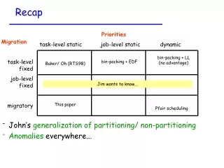
Recap Priorities task-level static job-level static dynamic Migration task-level fixed job-level fixed migratory bin-packing + LL (no advantage) bin-packing + EDF Baker/ Oh (RTS98) Jim wants to know... This paper Pfair scheduling • John’s generalization of partitioning/ non-partitioning • Anomalies everywhere...
This paper -I • Obs 1 & 2: increasing period may reduce feasibility • (reason: parallelism of processor left over by higher-pri tasks increases) • Obs 3: Critical instant not easily identified • Obs 4: Response time of a task depends upon relative priorities of higher-priority tasks • ==> the Audsley technique of priority assignment cannot be used
Finally, a non-anomalous result (Liu & Ha, 1994) Aperiodic jobs: Ji = (ai, ei) (not periodic tasks) • arrival time • execution requirement A system: • {J1, J2,...,Jn} • m processors • specified priorities • Let Fi denote the completion time of Ji Any system • {J1’, J2’,...,Jn’} with ei’ ei • m processors • the same priorities • let Fi’ denote the completion time of Ji’. Fi’ Fi can use for the middle column of our table, too!
This paper -II • Obs 1 & 2: increasing period may reduce feasibility • (reason: parallelism of processor left over by higher-pri tasks increases) • Obs 3: Critical instant not easily identified • Obs 4: Response time of a task depends upon relative priorities of higher-priority tasks • ==> the Audsley technique of priority assignment cannot be used • Theorem 1: A sufficient condition for feasibility • idea of the proof • possible problems (as pointed out by Phil)?
Theorem 1, corrected If for each i =(Ti, Ci) there exists an Li Ti such that [Ci + (SUM j : j hp(i) : (Li/Tj + 1) Cj) / m] Li then the task set is non-partition schedulable. Proof
A priority assignment scheme RM-US(1/4) • all tasks i with (Ti/ Ci > 1/4) have highest priorities • for the remaining tasks, rate-monotonic priorities Lemma: Any task system satisfying [ (SUM j : j : Ci /Ti) m/4] and [ (ALL j : j : Ci /Ti) 1/4] is successfully scheduled using RM-US(1/4) Theorem: Any task system satisfying [ (SUM j : j : Ci /Ti) m/4] is successfully scheduled using RM-US(1/4)
What this result means... Priorities task-level static job-level static dynamic Migration task-level fixed job-level fixed migratory bin-packing + LL (no advantage) bin-packing + EDF Baker/ Oh (RTS98) Pfair scheduling • First non-zero utilization bound for non-partitioning static-priority • Compare to partitioning (Baker & Oh) -- 41% • Room for improvement (simple algebra, perhaps ) • Exploit the non-anomaly of Liu & Ha to design job-levelstatic priority algorithms)
Resource augmentation and on-line scheduling on multiprocessors Phillips, Stein, Torng, and Wein. Optimal time-critical scheduling via resource augmentation. STOC (1997). Algorithmica (to appear).
Model and definitions Instance I = {J1, J2, ..., Jn} of jobs Jj = (rj, pj, wj, dj); (I) = max {pj} / min {pj} Known to be (off-line) feasible on m identical multiprocessors But the jobs revealed on line... An s-speed algorithm: meet all deadlines on m processors each s times as fast A w-machine algorithm: meet all deadlines on w m procs (each of the same speed as the original procs.)
Summary of results: Speed An s-speed algorithm: meet all deadlines on m processors each s times as fast EDF & LL are both (2 - 1/m)-speed algorithms • bound is tight for EDF Implies: twice as many processors ==> get optimal performance No 6/5 -speed algorithm can exist (on 2 procs)
Summary of results: machines A w-machine algorithm: meet all deadlines on w m procs (each of the same speed as the original procs.) LL is an O(log )-machine algorithm • not a c-machine algorithm for any constant c EDF is not an o()-machine algorithm “explains” difference between X-proc EDF & LL No 5/4 -machine algorithm can exist (on 2 procs)
The big insight: speed Definitions: A(j,t) denotes amount of execution of job j by Algorithm A until time t A(I,t) = [SUM: j I: A(j,t)] Let A be any “busy” (work-conserving) scheduling algorithm executing on processors of speed 1. What is the smallest such that at all times t, A(I, t) A’(I,t) for any other algorithm A’ executing on speed-1 processors? Lemma 2.6: turns out to be (2 - 1/m)/ • Thus, choosing equal to (2 - 1/m) gives = 1 (Choosing greater than this ( < 1) makes no physical sense) Use Lemma 2.6, and individual algorithm’s scheduling rules, to draw conclusions regarding these algorithms