1. 4.1 periodic sampling 4.2 discrete-time processing of continuous-time signals 4.3 continuous-time processing of discrete-time signal 4.4 digital processing of analog signals 4.5 changing the sampling rate using discrete-time processing Chapter 4 sampling of continous-time signals

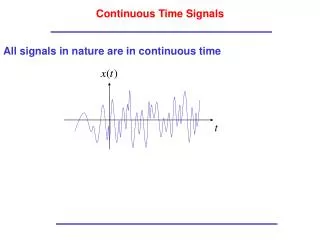
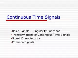
2. 4.1 periodic sampling1.ideal sample T：sample period fs=1/T:sample rate Ωs=2π/T:sample rate

3. Figure 4.1ideal continous-time-to-discrete-time(C/D)converter

4. time normalization tt/T=n Figure 4.2(a) mathematic model for ideal C/D

5. Figure 4.3 frequency spectrum change of ideal sample No aliasing aliasing aliasing frequency

6. Period =2πin time domain： w=2.1πand w=0.1πare the same trigonometric function property

7. high frequency is changed into low frequency in time domain：w=1.1π and w=0.9πare the same trigonometric function property

8. 2.ideal reconstruction Figure 4.10(b) ideal D/C converter

9. ideal reconstruction in frequency domain Figure 4.4

10. Take sinusoidal signal for example to understand aliasing from frequency domain EXAMPLE Figure 4.5

11. EXAMPLE Sampling frequency:8Hz Reconstruct frequency:

12. Figure 4.10(a) mathematic model for ideal D/C

13. ideal reconstruction in time domain

14. EXAMPLE Figure 4.9

15. understand aliasing from time-domain interpolation EXAMPLE

16. 3.Nyquist sampling theorems

17. Nyquist sampling theorems:

18. Figure 4.41 Digital processing of analog signals

19. examples of sampling theorem（1） The highest frequency of analog signal ,which wav file with sampling rate 16kHz can show ， is： 8kHz The higher sampling rate of audio files, the better fidelity.

21. examples of sampling theorem（2） according to what you know about the sampling rate of MP3 file，judge the sound we can feel frequency range（ ） （A）20~44.1kHz （B）20~20kHz （C）20~4kHz （D）20~8kHz B

22. Matlab codes to realize interpolation EXAMPLE

23. T=0.1; n=0:10; x=cos(10*pi*n*T); stem(n,x); dt=0.001; t=ones(11,1)* [0:dt:1]; n=n'*ones(1,1/dt+1); y=x*sinc((t-n*T)/T); hold on; plot(t/T,y,'r')

24. Supplement: band-pass sampling theorem：

27. 4.1 summary 1.representation in time domain of sampling

28. 2.changes in frequency domain caused by sampling

29. 3. understand reconstruction in frequency domain

30. 4. understand reconstruction in time domain

31. 5. sampling theorem

32. Requirements and difficulties： frequency spectrum chart of sampling and reconstruction comprehension and application of sampling theorem

33. Figure 4.11 4.2 discrete-time processing of continuous-time signals

34. Figure 4.12 conditions：LTI；no aliasing or aliasing occurred outside the pass band of filters EXAMPLE

35. EXAMPLE aliasing occurred outside the pass band of digital filters satisfies the equivalent relation of frequency response mentioned before. Figure 4.13

36. Figure 4.16 4.3 continuous-time processing of discrete-time signal

37. c Figure 4.12

38. EXAMPLE Ideal delay system：noninteger delay

39. quantization and coding Figure 4.41 4.4 digital processing of analog signals

40. Sampling and holding Figure 4.46(b)

41. uniform quantization and coding Figure 4.48

42. Figure 4.51 quantization error of 3BIT quantization error of8BIT

43. nonuniform quantization

44. 一维信号例子： index0 x 4 4 3 3 3 3 3 2 2 1 1 d(x,c0)=5 d(x,c1)=11 d(x,c2)=8 d(x,c3)=8 codewordc1 1 codeword c0 x 4 4 3 3 2 2 1 codewordc2 codewordc3 1 码书 vector quantization

45. Example: image coding • Initial image block（4 gray-levels，dimentions k=4×4=16） x 0 1 2 3 Code book C ＝｛y0, y1 , y2, y3｝ y0 y1 y2 y3 codeword y1 is the most adjacent to x，so it is coded by the index “01”. d(x,y0)=25 d(x,y1)=5 d(x,y2)=25 d(x,y3)=46 vector quantization

46. reconstruction Figure 4.53 D/A过程

47. Figure 4.5

48. record the digital sound

49. Influence caused by sampling rate and quantizing bits

50. Different tones require different sampling rates.