Download
1 / 64
710 likes | 1.51k Vues
Chapter 7 Linear Programming Models: Graphical and Computer Methods. Prepared by Lee Revere and John Large. Learning Objectives. Students will be able to: Understand the basic assumptions and properties of linear programming (LP).

E N D
Chapter 7 Linear Programming Models: Graphical and Computer Methods Prepared by Lee Revere and John Large 7-1
Learning Objectives Students will be able to: • Understand the basic assumptions and properties of linear programming (LP). • Graphically solve any LP problem that has only two variables by both the corner point and isoprofit line methods. • Understand special issues in LP such as infeasibility, unboundedness, redundancy, and alternative optimal solutions. • Understand the role of sensitivity analysis. • Use Excel spreadsheets to solve LP problems. 7-2
Chapter Outline 7.1 Introduction 7.2 Requirements of a Linear Programming Problem 7.3 Formulating LP Problems 7.4 Graphical Solution to an LP Problem 7.5 Solving Flair Furniture’s LP Problem using QM for Windows and Excel 7.6 Solving Minimization Problems 7.7 Four Special Cases in LP 7.8 Sensitivity Analysis 7-3
Introduction Linear programming(LP) is • a widely used mathematical modeling technique • designed to help managers in planning and decision making • relative to resource allocation. • LPis a technique that helps in resource allocation decisions. Programmingrefers to • modeling and solving a problem mathematically. 7-4
Examples of Successful LP Applications 1.Development of a production schedule that will • satisfy future demands for a firm’s production • while minimizing total production and inventory costs 2. Selection of product mix in a factory to • make best use of machine-hours and labor-hours available • while maximizing the firm’s products 7-5
Examples of Successful LP Applications(continued) 3.Determination of grades of petroleum products to yield the maximum profit 4. Selection of different blends of raw materials to feed mills to produce finished feed combinations at minimum cost 5. Determination of a distribution system that will minimize total shipping cost from several warehouses to various market locations 7-6
Requirements of a Linear Programming Problem All LP problems have 4 properties in common: • All problems seek to maximize or minimize some quantity (the objective function). • The presence of restrictions or constraints limits the degree to which we can pursue our objective. • There must be alternative courses of action to choose from. • The objective and constraints in linear programming problems must be expressed in terms of linear equations or inequalities. 7-7
5 Basic Assumptions of Linear Programming • Certainty: • numbers in the objective and constraints are known with certainty and do not change during the period being studied • Proportionality: • exists in the objective and constraints • constancy between production increases and resource utilization • Additivity: • the total of all activities equals the sum of the individual activities 7-8
5 Basic Assumptions of Linear Programming (continued) • Divisibility: • solutions need not be in whole numbers (integers) • solutions are divisible, and may take any fractional value • Non-negativity: • all answers or variables are greater than or equal to (≥) zero • negative values of physical quantities are impossible 7-9
Formulating Linear Programming Problems • Formulating a linear program involves developing a mathematical model to represent the managerial problem. • Once the managerial problem is understood, begin to develop the mathematical statement of the problem. • The steps in formulating a linear program follow on the next slide. 7-10
Formulating Linear Programming Problems (continued) Steps in LP Formulations 1.Completely understand the managerial problem being faced. 2.Identify the objective and the constraints. 3.Define the decision variables. 4.Use the decision variables to write mathematical expressions for the objective function and the constraints. 7-11
Formulating Linear Programming Problems (continued) The Product Mix Problem • Two or more products are usually produced using limited resources such as - personnel, machines, raw materials, and so on. • The profit that the firm seeks to maximize is based on the profit contribution per unit of each product. • The company would like to determine how many units of each product it should produce so as to maximize overall profit given its limited resources. • A problem of this type is formulated in the following example on the next slide. 7-12
Flair Furniture Company Data - Table 7.1 Available Hours This Week T Tables C Chairs Department • Carpentry • Painting • &Varnishing 4 2 3 1 240 100 Hours Required to Produce One Unit Mathematical formulation: Profit Amount $7 $5 Constraints: 4T + 3C 240 (Carpentry) 2T + 1C 100 (Paint & Varnishing) T ≥ 0 (1st nonnegative cons) C ≥ 0 (2nd nonnegative cons) Max. Objective, z: 7T + 5C 7-13
Flair Furniture Company Constraints The easiest way to solve a small LP problem, such as that of the Flair Furniture Company, is with the graphical solution approach. The graphical method works only when there are two decision variables, but it provides valuable insight into how larger problems are structured. When there are more than two variables, it is not possible to plot the solution on a two-dimensional graph; a more complex approach is needed. But the graphical method is invaluable in providing us with insights into how other approaches work. 7-14
Flair Furniture Company Constraints 120 100 80 60 40 20 0 Painting/Varnishing Number of Chairs Carpentry 20 40 60 80 100 2T + 1C ≤ 100 4T + 3C ≤ 240 Number of Tables 7-15
Flair Furniture Company Feasible Region 120 100 80 60 40 20 0 Painting/Varnishing Number of Chairs Carpentry Feasible Region 20 40 60 80 100 Number of Tables 7-16
Isoprofit Lines Steps 1. Graph all constraints and find the feasible region. 2. Select a specific profit (or cost) line and graph it to find the slope. 3. Move the objective function line in the direction of increasing profit (or decreasing cost) while maintaining the slope. The last point it touches in the feasible region is the optimal solution. 4. Find the values of the decision variables at this last point and compute the profit (or cost). 7-17
Flair Furniture Company Isoprofit Lines Isoprofit Line Solution Method • Start by letting profits equal some arbitrary but small dollar amount. • Choose a profit of, say, $210. - This is a profit level that can be obtained easily without violating either of the two constraints. • The objective function can be written as $210 = 7T + 5C. 7-18
Flair Furniture Company Isoprofit Lines Isoprofit Line Solution Method • The objective function is just the equation of a line called an isoprofit line. - It represents all combinations of (T, C) that would yield a total profit of $210. • To plot the profit line, proceed exactly as done to plot a constraint line: - First, let T = 0 and solve for the point at which the line crosses the C axis. - Then, let C = 0 and solve for T. • $210 = $7(0) + $5(C) • C = 42 chairs • Then, let C = 0 and solve for T. • $210 = $7(T) + $5(0) • T = 30 tables 7-19
Flair Furniture Company Isoprofit Lines Isoprofit Line Solution Method • Next connect these two points with a straight line. This profit line is illustrated in the next slide. • All points on the line represent feasible solutions that produce an approximate profit of $210 • Obviously, the isoprofit line for $210 does not produce the highest possible profit to the firm. • Try graphing more lines, each yielding a higher profit. • Another equation, $420 = $7T + $5C, is plotted in the same fashion as the lower line. 7-20
Flair Furniture Company Isoprofit Lines Isoprofit Line Solution Method • When T = 0, • $420 = $7(0) + 5(C) • C = 84 chairs • When C = 0, • $420 = $7(T) + 5(0) • T = 60 tables • This line is too high to be considered as it no longer touches the feasible region. • The highest possible isoprofit line is illustrated in the second following slide. It touches the tip of the feasible region at the corner point (T = 30, C = 40) and yields a profit of $410. 7-21
Flair Furniture Company Isoprofit Lines 120 100 80 60 40 20 0 Painting/Varnishing 7T + 5C = 210 Number of Chairs 7T + 5C = 420 Carpentry 20 40 60 80 100 Number of Tables 7-22
Flair Furniture Company Optimal Solution Isoprofit Lines 120 100 80 60 40 20 0 Painting/Varnishing Solution (T = 30, C = 40) Number of Chairs Carpentry 20 40 60 80 100 Number of Tables 7-23
Flair Furniture Company Corner Point Corner Point Solution Method • A second approach to solving LP problems • It involves looking at the profit at every corner point of the feasible region • The mathematical theory behind LP is that the optimal solution must lie at one of the corner points in the feasible region 7-24
Corner Point Corner Point Solution Method, Summary 1. Graph all constraints and find the feasible region. 2. Find the corner points of the feasible region. 3. Compute the profit (or cost) at each of the feasible corner points. 4. Select the corner point with the best value of the objective function found in step 3. This is the optimal solution. 7-25
Flair Furniture Company Corner Point Corner Point Solution Method • The feasible region for the Flair Furniture Company problem is a four-sided polygon with four corner, or extreme, points. • These points are labeled 1 ,2 ,3 , and 4 on the next graph. • To find the (T, C) values producing the maximum profit, find the coordinates of each corner point and test their profit levels. Point 1:(T = 0,C = 0) profit = $7(0) + $5(0) = $0 Point 2:(T = 0,C = 80) profit = $7(0) + $5(80) = $400 Point 3:(T = 30,C = 40) profit = $7(30) + $5(40) = $410 Point 4 : (T = 50, C = 0) profit = $7(50) + $5(0) = $350 7-26
Flair Furniture Company Optimal Solution Corner Points 120 100 80 60 40 20 0 2 Painting/Varnishing Solution (T = 30, C = 40) Number of Chairs Carpentry 3 1 4 20 40 60 80 100 Number of Tables 7-27
Flair Furniture - QM for Windows • To use QM for Windows, • Select the Linear Programming module. • Then specify - the number of constraints (other than the non-negativity constraints, as it is assumed that the variables must be nonnegative), - the number of variables, and - whether the objective is to be maximized or minimized. • For the Flair Furniture Company problem, there are • two constraints and two variables. • Once these numbers are specified, the input window opens as shown on the next slide. 7-28
Flair Furniture - QM for Windows(continued) • Next, the coefficients for the objective function and the constraints can be entered. - Placing the cursor over the X1 or X2 and typing a new name such as Tables and Chairs will change the variable names. - The constraint names can be similarly modified. - When you select the Solve button, you get the output shown in the next slide. 7-29
Flair Furniture - QM for Windows (continued) • Modify the problem by selecting the Edit button and returning to the input screen to make any desired changes. • Once these numbers are specified, the input window opens as shown on the next slide. • Once the problem has been solved, a graph may be displayed by selecting Window—Graph from the menu bar in QM for Windows. • The next slide shows the output for the graphical solution. • Notice that in addition to the graph, the corner points and the original problem are also shown. 7-31
Flair Furniture – Solver in Excel • To use Solver, open an Excel sheet and: • Enter the variable names and the coefficients for the objective function and constraints. • Specify cells where the values of the variables will be located. The solution will be put here. • Write a formula to compute the value of the objective function. The SUMPRODUCT function is helpful with this. • Write formulas to compute the left-hand sides of the constraints. Formulas may be copied and pasted to these cells. • Indicate constraint signs (≤, =, and ≥) for display purposes only. The actual signs must be entered into Solver later, but having these displayed in the spreadsheet is helpful. • Input the right-hand side values for each constraint. 7-33
Flair Furniture – Solver in Excel (continued) • Once the problem is entered in an Excel sheet, follow these steps to use Solver: • In Excel, select Tools—Solver. • If Solver does not appear on the menu under Tools, select Tools—Add-ins and then check the box next to Solver Add-in. Solver then will display in the Tools drop-down menu. • Once Solver has been selected, a window will open for the input of the Solver Parameters. Move the cursor to the Set Target Cell box and fill in the cell that is used to calculate the value of the objective function. • Move the cursor to the By Changing Cells box and input the cells that will contain the values for the variables. • Move the cursor to the Subject to the Constraints box, and then select Add. 7-34
Flair Furniture – Solver in Excel (continued) • Solver steps, continued: • The Cell Reference box is for the range of cells that contain the left-hand sides of the constraints. • Select the ≤ to change the type of constraint if necessary. Since this setting is the default, no change is necessary. • If there had been some ≥ or = constraints in addition to the ≤ constraints, you would have to input all of one type [e.g., ≤] first, and then select Add to input the other type of constraint. • Move the cursor to the Constraint box to input the right-hand sides of the constraints. Select Add to finish this set of constraints and begin inputting another set, or select OK if there are no other constraints to add. 7-35
Flair Furniture – Solver in Excel (continued) • Solver steps, continued: • From the Solver Parameters window, select Options and check Assume Linear Model and check Assume Non-negative; then click OK. • Review the information in the Solver window to make sure it is correct, and click Solve. • The Solver Solutions window is displayed and indicates that a solution was found. The values for the variables, the objective function, and the slacks are shown also. • Select Keep Solver Solution and the values in the spreadsheet will be kept at the optimal solution. • You may select what sort of additional information (e.g., Sensitivity) is to be presented from the reports Window (discussed later). You may select any of these and select OK to have these automatically generated. 7-36
Flair Furniture – Solver in Excel(continued) • On the next slide is an example of the type of worksheet used in Excel for Solver. • The worksheet demonstrates some of the steps previously discussed. 7-37
Solving Minimization Problems Many LP problems minimize an objective, such as cost, instead of maximizing a profit function. For example, • A restaurant may wish to develop a work schedule to meet staffing needs while minimizing the total number of employees. Or, • A manufacturer may seek to distribute its products from several factories to its many regional warehouses in such a way as to minimize total shipping costs. Or, • A hospital may want to provide a daily meal plan for its patients that meets certain nutritional standards while minimizing food purchase costs. 7-39
Solving Minimization Problems Minimization problems can be solved graphically by • first setting up the feasible solution region and then using either • the corner point method or • an isocost line approach (which is analogous to the isoprofit approach in maximization problems) to find the values of the decision variables (e.g., X1 and X2) that yield the minimum cost. 7-40
Solving Minimization Problems Holiday Meal Turkey Ranch example Minimize: 2X1 + 3X2 Subject to: 5X1 + 10X2³ 90 oz. (A) 4X1 + 3X2³ 48 oz. (B) ½ X1³ 1 ½ oz. (C) X1, X2³ 0 (D) where, X 1 = # of pounds of brand 1 feed purchased X 2 = # of pounds of brand 2 feed purchased (A) = ingredient A constraint (B) = ingredient B constraint (C) = ingredient C constraint (D) = non-negativity constraints 7-41
Holiday Meal Turkey Ranch • Using the Corner Point Method • To solve this problem: • Construct the feasible solution region. • This is done by plotting each of the three constraint equations. • Find the corner points. • This problem has 3 corner points, labeled a, b, and c. - Minimization problems are often unbound outward (i.e., to the right and on top), but this causes no difficulty in solving them. - As long as they are bounded inward (on the left side and the bottom), corner points may be established. - The optimal solution will lie at one of the corners as it would in a maximization problem. 7-42
Holiday Meal Turkey Problem Corner Points 7-43
Solving Minimization Problems Using the Isocost Line Approach • As with isoprofit lines, there is no need to compute the cost at each corner point, but instead draw a series of parallel cost lines. • The lowest cost line (i.e., the one closest in toward the origin) to touch the feasible region provides the optimal solution corner. • Start, for example, by drawing a 54-cent cost line, namely 54 = 2X1 + 3X2. - Obviously, there are many points in the feasible region that would yield a lower total cost. 7-44
Solving Minimization Problems (continued) • Proceed to move the isocost line toward the lower left, in a plane parallel to the 54-cent solution line. • The last point touched while still in contact with the feasible region is the same as corner point b of the Corner Point diagram in the previous slide. - It has the coordinates (X1 = 8.4, X2 = 4.8) and an associated cost of 31.2 cents. 7-45
Holiday Meal Turkey Problem Isoprofit Lines 7-46
Special Cases in LP Four special cases and difficulties arise at times when solving LP problems: • Infeasibility: - lack of a feasible solution region can occur if constraints conflict with one another. • Unbounded Solutions: - when the objective function in a maximization problem can be infinitely large, the problem is unbounded and is missing one or more constraints. • Redundancy: - a redundant constraint is one that does not affect the feasible solution region. • More than One Optimal Solution: • two or more optimal solutions may exist, and • this actually allows management great flexibility in deciding which combination to select. 7-47
A Problem with No Feasible Solution X2 8 6 4 2 0 Region Satisfying 3rd Constraint 2 4 6 8 X1 Region Satisfying First 2 Constraints 7-48
A Solution Region That is Unbounded to the Right X2 X1 > 5 15 10 5 0 X2 < 10 Feasible Region X1 +2X2 > 10 5 10 15 X1 7-49
A Problem with a Redundant Constraint X2 30 25 20 15 10 5 0 Redundant Constraint 2X1 + X2 < 30 X1 < 25 X1 +X2 < 20 Feasible Region X1 5 10 15 20 25 30 7-50