Hypothesis and Hypothesis Testing
This guide explores the fundamental concepts of hypothesis testing, a procedure used to assess assumptions about a population parameter using sample evidence and probability theory. It clarifies the roles of null (H0) and alternative (H1) hypotheses, significance levels, test statistics, and critical values. Readers will learn about one-tailed and two-tailed tests, the importance of significance levels (α), and common types of errors. Examples illustrate how to formulate hypotheses, calculate test statistics, and make informed decisions based on statistical analysis.

Hypothesis and Hypothesis Testing
E N D
Presentation Transcript
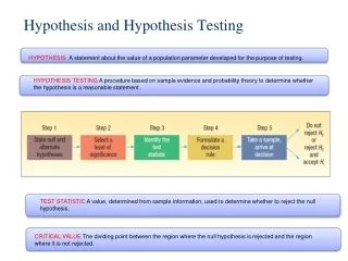
HYPOTHESIS A statement about the value of a population parameter developed for the purpose of testing. Hypothesis and Hypothesis Testing HYPOTHESIS TESTING A procedure based on sample evidence and probability theory to determine whether the hypothesis is a reasonable statement. TEST STATISTIC A value, determined from sample information, used to determine whether to reject the null hypothesis. CRITICAL VALUE The dividing point between the region where the null hypothesis is rejected and the region where it is not rejected.
Important Things to Remember about H0 and H1 • H0: null hypothesis and H1: alternate hypothesis • H0 and H1 are mutually exclusive and collectively exhaustive • H0 is always presumed to be true • H1 is the research hypothesis • A random sample (n) is used to “reject H0” • If we conclude 'do not reject H0', this does not necessarily mean that the null hypothesis is true, it only suggests that there is not sufficient evidence to reject H0; rejecting the null hypothesis then, suggests that the alternative hypothesis may be true. • Equality is always part of H0 (e.g. “=” , “≥” , “≤”). • “≠” “<” and “>” always part of H1 • In actual practice, the status quo is set up as H0 • In problem solving, look for key words and convert them into symbols. Some key words include: “improved, better than, as effective as, different from, has changed, etc.”
Two-tailed Test Two-tailed tests - the rejection region is in both tails of the distribution Rejection Region Rejection Region Acceptance Region One-tailed tests - the rejection region is in only on one tail of the distribution One-tailed Test Rejection Region Acceptance Region
Types of Errors is true is false Type I error P(Type I)= Correct Decision Reject Type II error P(Type II)= Correct Decision Do not reject Type I Error - Defined as the probability of rejecting the null hypothesis when it is actually true. This is denoted by the Greek letter “” Also known as the significance level of a test Type II Error: Defined as the probability of “accepting” the null hypothesis when it is actually false. This is denoted by the Greek letter “β”
Hypothesis Setups for Testing a Mean () or a Proportion () MEAN PROPORTION
Steps in hypothesis testing - Define Null hypothesis - Define Alternative hypothesis - Calculate Test statistic - Determine Rejection region • Compare Value of the test statistic with Critical Value - Conclusion
Testing for a Population Mean with aKnown Population Standard Deviation- Example Step 4: Formulate the decision rule. Reject H0 if |Z| > Z/2 Step 5: Make a decision and interpret the result. Because 1.55 does not fall in the rejection region, H0 is not rejected. Weconclude that the population mean is not different from 200. So we wouldreport to the vice president of manufacturing that the sample evidence doesnot show that the production rate at the plant has changed from200 per week. EXAMPLE Jamestown Steel Company manufactures and assembles desks and other office equipment . The weekly production of the Model A325 desk at the Fredonia Plant follows the normal probability distribution with a mean of 200 and a standard deviation of 16. Recently, new production methods have been introduced and new employees hired. The mean number of desks produced during last 50 weeks was 203.5. The VP of manufacturing would like to investigate whether there has been a changein the weekly production of the Model A325 desk, at 1% level of significance. Step 1: State the null hypothesis and the alternate hypothesis. H0: = 200 H1: ≠ 200 (note: This is a 2-tail test, as the keyword in the problem “has changed”) Step 2: Select the level of significance. α = 0.01 as stated in the problem Step 3: Select the test statistic. Use Z-distribution since σ is known
Testing for a Population Mean with a Known Population Standard Deviation- Another Example Step 4: Formulate the decision rule. Reject H0 if Z > Z Step 5: Make a decision and interpret the result. Because 1.55 does not fall in the rejection region, H0 is not rejected. Weconclude that the average number of desks assembled in the last 50 weeks is not more than 200 Suppose in the previous problem the vice president wants to know whether there has been an increase in the number of units assembled. To put it another way, can we conclude, because of the improved production methods, that the mean number of desks assembled in the last 50 weeks was more than 200? Recall: σ=16, =200, α=.01 Step 1: State the null hypothesis and the alternate hypothesis. H0: ≤ 200 H1: > 200 (note: This is a 1-tail test as the keyword in the problem “an increase”) Step 2: Select the level of significance. α = 0.01 as stated in the problem Step 3: Select the test statistic. Use Z-distribution since σ is known
p-value in Hypothesis Testing EAMPLE p-Value Recall the last problem where the hypothesis and decision rules were set up as: H0: ≤ 200 H1: > 200 Reject H0 if Z > Z where Z = 1.55 and Z =2.33 Reject H0 if p-value < 0.0606 is not < 0.01 Conclude: Fail to reject H0 • p-VALUEis the probability of observing a sample value as extreme as, or more extreme than, the value observed, given that the null hypothesis is true. • In testing a hypothesis, we can also compare the p-value tothe significance level (). • Decision rule using the p-value: Reject null hypothesis, if p<α
Interpreting the p-value • Describing the p-value • If the p-value is less than 1%, there is overwhelming evidence that supports the alternative hypothesis. • If the p-value is between 1% and 5%, there is a strong evidence that supports the alternative hypothesis. • If the p-value is between 5% and 10% there is a weak evidence that supports the alternative hypothesis. • If the p-value exceeds 10%, there is no evidence that supports the alternative hypothesis.
The Power of Statistical Test The power of a statistical test, given as 1 –b = P (reject H0 when H0 is false), measures the ability of the test to perform as required. This 1 –b is called the power of the function. This means that greater the power of the function the better would be the decision rule. There are two types of tail test 1. One-tailed tests - the rejection region is in only one tail of the distribution 2. Two-tailed tests - the rejection region is in both tails of the distribution
Steps in Hypothesis Testing using SPSS • State the null and alternative hypotheses • Define the level of significance (α) • Calculate the actual significance : p-value • Make decision : Reject null hypothesis, if p≤ α, for 2-tail test; and if p*≤ α, for 1-tail test.(p* is p/2 when p is obtained from 2-tail test) • Conclusion
Inference About a Population Mean When the Population Standard Deviation Is Unknown or When the Sample Size is Small In practice, the population standard deviation will be unknown. Recall that when sis known we use the following statistic to estimate and test a population mean When sis unknown or when the sample size is small, we use its point estimator s, and the z-statistic is replaced then by the t-statistic
The t - Statistic t s The “degrees of freedom”, (a function of the sample size) determine how spread the distribution is (compared to the normal distribution) The t distribution is mound-shaped, and symmetrical around zero. d.f. = v2 d.f. = v1 v1 < v2 0
Testing m when s is unknown • Example • In order to determine the number of workers required to meet demand, the productivity of newly hired trainees is studied. • It is believed that trainees can process and distribute more than 450 packages per hour within one week of hiring. • Can we conclude that this belief is correct, based on productivity observation of 50 trainees (see file PROD.sav).
Testing m when s is unknown • Example – Solution • The problem objective is to describe the population of the number of packages processed in one hour. • H0:m = 450 H1:m > 450 • The t statistic d.f. = n - 1 = 49
Testing m when s is unknown • Solution continued (solving by hand) • The rejection region is t > ta,n – 1ta,n - 1 = t.05,49 @ t.05,50 = 1.676.
Testing m when s is unknown Rejection region • The test statistic is 1.676 1.89 • Since 1.89 > 1.676 we reject the null hypothesis in favor of the alternative. • There is sufficient evidence to infer that the mean productivity of trainees one week after being hired is greater than 450 packages at .05 significance level.
Under certain conditions, [np > 5 and n(1-p) > 5], is approximately normally distributed, with m = p and s2 = p(1 - p)/n. Inference About a Population Proportion • Statistic and sampling distribution • the statistic used when making inference about p is:
Testing and Estimating the Proportion • Test statistic for p
Testing the Proportion • Example 12.6 • A pharmaceutical company claimed that its medicine was 80% effective in relieving allergy. In a sample of 200 persons, who were given medicine only 150 persons had relief. Do you thank that the effectiveness is below 80%? Use 0.05 level of significance.
Testing the Proportion • Solution • The problem objective is to test the effectiveness of medicine. • The data are nominal. • The parameter to be tested is ‘p’. • Success is defined as “having relief”. • The hypotheses are: H0: p = .8 H1: p < .8
Testing the Proportion • Solution • The rejection region is z < za = z.05 = -1.645. • The sample proportion is • The value of the test statistic is Since calculated z is less than critical value, we reject null hypothesis and conclude that the claim of the company that its medicine is 80% effective is not justified.
T-Tests : When sample size is small (<30) or When the Population Standard Deviation Is Unknown • Variable : Normal • Types of t-tests: One-sample t-test Paired or dependent sample t-test Independent samples t-test (Equal and Unequal Variance)
Matched pairs The mean of the population differences is that is Test statistic: Degree of freedom =
The sampling process. Population2 Population 1 Parameters: Parameters: Statistics: Statistics: Sample size: Sample size:
If the two population standard deviations are unknown, then we can estimate the standard error of the difference between two means.
If population variance unknown and the sample size is small and the population variances are equal Then we will use the weighted average called a “ pooled estimate” of Where:
Test statistic: Degree of freedom =
One way Analysis of Variance ( ANOVA ) ANOVA is a technique used to test a hypothesis concerning the means of three or more populations.
Comparing Means of Three or More Populations The F distribution is used for testing whether two or more sample means came from the same or equal populations. Assumptions: • The sampled populations follow the normal distribution. • The populations have equal standard deviations. • The samples are randomly selected and are independent. TheNull Hypothesis is that the population means are the same. The Alternative Hypothesis is that at least one of the means is different. H0: µ1 = µ2 =…= µk H1: The means are not all equal Reject H0 if F > F,k-1,n-k
The test statistic used to test the hypothesis is F statistic Assumptions: 1. The random variable is normally distributed. 2. The population variances are equal.
ANOVA – Example (File Airlines.sav) EXAMPLE Recently a group of four major carriers joined in hiring Brunner Marketing Research, Inc., to survey recent passengers regarding their level of satisfaction with a recent flight. The survey included questions on ticketing, boarding, in-flight service, baggage handling, pilot communication, and so forth. Twenty-five questions offered a range of possible answers: excellent, good, fair, or poor. A response of excellent was given a score of 4, good a 3, fair a 2, and poor a 1. These responses were then totaled, so the total score was an indication of the satisfaction with the flight. Brunner Marketing Research, Inc., randomly selected and surveyed passengers from the four airlines. Is there a difference in the mean satisfaction level among the four airlines? Use the .01 significance level. Step 1: State the null and alternate hypotheses. H0: µE = µA = µT = µO H1: The means are not all equal Reject H0 if F > F,k-1,n-k Step 2: State the level of significance. The .01 significance level is stated in the problem.
ANOVA – Example Step 3: Find the appropriate test statistic. Use the F statistic Calculations: It is convenient to summarize the calculations of F statistic in an ANOVA Table.
ANOVA – Example Compute the value of F and make a decision We find deviation of each observation from the grand mean, square the deviations, and sum this result for all 22 observations. SS total = {(94-75.64)2 + (90-75.64)2 + ……+(65-75.64)2 } = 1485.10 To compute SSE, find deviation between each observation and its treatment mean. Each of these values is squared and then summed for all 22 observations. SSE = {(94-87.25)2 + (90-87.25)2 + ……+(80-87.25)2 } + {(75-78.20)2 + (68-78.20)2 + ……+(88-78.20)2 } + {(70-72.86)2 + (73-72.86)2 + ……+(65-72.86)2 } + {(68-69)2 + (70-69)2 + ……+(65-69)2 } = 594.41 Finally, determine SST = SS total – SSE. SST = 1485.10 – 594.41 = 890.69
ANOVA – Example Step 3: Find the appropriate test statistic. Use the F statistic Calculations: It is convenient to summarize the calculations of F statistic in an ANOVA Table. Step 4: State the decision rule. Reject H0 if: F > F,k-1,n-k F > F.01,4-1,22-4 F > F.01,3,18 F > 5.09 Step 5: Make a decision. The computed value of F is 8.99, which is greater than the critical value of 5.09, so the null hypothesis is rejected. Conclusion: The mean scores are not the same for the four airlines; at this point we can only conclude there is a difference in the treatment means. We cannot determine which treatment groups differ or how many treatment groups differ.
ANOVA Example – SPSS Output Homogeneous Subsets
Chi-squared Test of a Contingency Table • Test of Independence : Test on association between two nominal variables regarding contingency tables. Null Hypothesis : Two variables are independent Alternative Hypothesis : The two variables are dependent
The Chi-square Distribution At the outset, we should know that the chi-square distribution has only one parameter called the ‘degrees of freedom’ (df ) as is the case with the t-distribution. The shape of a particular chi-square distribution depends on the number of degrees of freedom.
Properties of Chi-square Distribution • Chi-square is non-negative in value; it is either zero or positively valued. • It is not symmetrical; it is skewed to the right. • There are many chi-square distributions. As with the t-distribution, there is a different chi-square distribution for each degree-of-freedom value.
The chi-squared statistic measures the difference between the actual counts and the expected counts ( assuming validity of the null hypothesis) ( Observed count - Expected count )2 The sum Expected count
Contingency table c2 test – Example • In an effort to better predict the demand for courses offered by a certain MBA program, it was hypothesized that students’ academic background affect their choice of MBA major, thus, their courses selection. • A random sample of last year’s MBA students was selected. The data is given in the file Chi-Sq_MBA.sav. • The following contingency table summarizes relevant data.