Download
1 / 35
350 likes | 582 Vues
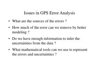
Issues in GPS Error Analysis. What are the sources of the errors ? How much of the error can we remove by better modeling ? Do we have enough information to infer the uncertainties from the data ? What mathematical tools can we use to represent the errors and uncertainties ? .

E N D
Issues in GPS Error Analysis • What are the sources of the errors ? • How much of the error can we remove by better modeling ? • Do we have enough information to infer the uncertainties from the data ? • What mathematical tools can we use to represent the errors and uncertainties ?
Determining the Uncertainties of GPS Estimates of Station Velocities • Rigorous estimate of uncertainties requires full knowledge of the error spectrum—both temporal and spatial correlations (never possible) • Sufficient approximations are often available by examining time series (phase and/or position) and reweighting data • Whatever the assumed error model and tools used to implement it, external validation is important
Sources of Error • Signal propagation effects • Receiver noise • Ionospheric effects • Signal scattering ( antenna phase center / multipath ) • Atmospheric delay (mainly water vapor) • Unmodeled motions of the station • Monument instability • Loading of the crust by atmosphere, oceans, and surface water • Unmodeled motions of the satellites
Simple geometry for incidence of a direct and reflected signal Multipath contributions to observed phase for an antenna at heights (a) 0.15 m, (b) 0.6 m, and (c ) 1 m. [From Elosegui et al, 1995]
Epochs 20 0 mm -20 1 2 3 4 5 Hours Elevation angle and phase residuals for single satellite
Figure 5 from Williams et al [2004]: Power spectrum for common-mode error in the SOPAC regional SCIGN analysis. Lines are best-fit WN + FN models (solid=mean ampl; dashed=MLE) Note lack of taper and misfit for periods > 1 yr
Characterizations of Time-series Noise • Power law: slope of line fit to spectrum • 0 = white noise • -1 = flicker noise • -2 = random walk • Non-integer spectral index (e.g. “fraction white noise” 1 > k > -1 ) • Good discussion in Williams [2003] • Problems: • No model captures reliably the lowest-frequency part of the spectrum • Noise is often non-stationary
Examples of times series and spectra for global stations From Mao et al., 1999
White noise vs flicker noise from Mao et al. [1999] spectral analysis of 23 global stations
“Realistic sigma” option on in tsview: rate sigmas and red lines now show based on the results of applying the algorithm.
“Realistic Sigma” Algorithm • Motivation: computational efficiency, handle time series with varying lengths and data gaps • Concept: The departure from a white-noise (sqrt n) reduction in noise with averaging provides a measure of correlated noise. • Implementation: • Fit the values of chi2 vs averaging time to a first-order Gauss-Markov (FOGM) process (amplitude, correlation time) • Use the chi2 value for infinite averaging time predicted from this model to scale the white-noise sigma estimates from the original fit and/or • Fit the values to a FOGM with infinite averaging time (i.e., random walk) and use these estimates as input to globk (mar_neu command)
Practical Approaches • White noise as a proxy for flicker noise [Mao et al., 1999] • White noise + flicker noise (+ random walk) to model the spectrum [Williams et al., 2004] • Random walk to model to model an exponential spectrum [Herring “realistic sigma algorithm”] • “Eyeball” white noise + random walk for non-continuous data ______________________________________ • Only the last two can be applied in GLOBK for velocity estimation • All approaches require common sense and verification
SARG 217U GOBS DALL BURN
SARG 217U GOBS DALL BURN
SARG 217U GOBS DALL BURN
SARG 217U GOBS DALL BURN
Percent Within Ratio Cumulative histogram of normalized velocity residuals for Eastern Oregon & Washington Noise added to position for each survey: 0.5 mm random 1.0 mm/sqrt(yr)) random walk Solid line is theoretical for Gaussian distribution Ratio (velocity magnitude/uncertainty)
Cumulative histogram of normalized velocity residuals for Eastern Oregon & Washington Noise added to position for each survey: 0.5 mm random 0.5 mm/yr random walk Solid line is theoretical for Gaussian distribution Percent Within Ratio Ratio (velocity magnitude/uncertainty)
Cumulative histogram of normalized velocity residuals for Eastern Oregon & Washington Noise added to position for each survey: 2.0 mm random 1.5 mm/yr random walk Solid line is theoretical for Gaussian distribution Percent Within Ratio Ratio (velocity magnitude/uncertainty)
Summary • All algorithms for computing estimates of standard deviations have various problems: Fundamentally, rate standard deviations are dependent on low frequency part of noise spectrum which is poorly determined. • Assumptions of stationarity are often not valid (example shown) • “Realistic sigma” algorithm implemented in tsview and enfit/ensum; sh_gen_stats generates mar_neu commands for globk based on the noise estimates
Globk re-weighting • There are methods in globk to change the standard deviations of the position (and other parameter) estimates. • Complete solutions: • In the gdl files, variance rescaling factor and diagonal rescaling factors can be added. • First factor scales the whole covariance matrix. Useful when • Using SINEX files from different programs • Accounting for different sampling rates • Second factor is not normally needed and is used to solve numerical instability problems. Scales diagonal of covariance matrix. • Needed in some SINEX files • Large globk combinations (negative chi-square increments) Large combinations are best done with pre-combinations in to weekly or monthly solutions • Individual sites with sig_neu command. Wild cards allowded in site names (both beginning and end)