Error Analysis

1. Chapter 4: Errors in measurements Error Analysis

2. Chapter 4: Errors in measurements Frequency distributions Suppose that the length of a steel bar is measured by a number of different observers and the following set of 23 measurements are recorded (units mm). 409,406, 402, 407, 405, 404, 407, 404, 407, 407, 408, 406, 410, 406, 405, 408, 406, 409, 406, 405, 409, 406, 407. • Draw the following: • Histogram of measurements and deviations • Gaussian distribution (Normal distribution)

3. Chapter 4: Errors in measurements Histogram of measurements and deviations

4. Chapter 4: Errors in measurements Gaussian distribution Measurement sets that only contain random errors usually conform to a distribution with a particular shape that is called Gaussian. The shape of a Gaussian curve is such that the frequency of small deviations from the mean value is much greater thanthe frequency of large deviations. This coincides with the usual expectation in measurements subject to random errors that the number of measurements with a small error is much larger than the number of measurements with a large error. Alternative names for the Gaussian distribution are the Normal distribution or Bell-shapeddistribution. A Gaussian curve is formally defined as a normalized frequency distribution that is symmetrical about the line of zero error and in which the frequency and magnitude of quantities are related by the expression:

5. Chapter 4: Errors in measurements F(x) xi F(d)

6. Chapter 4: Errors in measurements = - xtrue

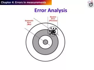
7. Chapter 8: Errors and Uncertainties Mechanical Eng. Dept. Bias Error (Systematic Error) Remains Constant During Test Estimated Based on Calibration Precision Error (Random Error) Precision index = Estimate of Standard deviation, 

8. Chapter 8: Errors and Uncertainties Mechanical Eng. Dept.

9. Chapter 4: Errors in measurements Estimation of Random Errors They are represented by repeatability described in earlier lectures. Repeatability (R) is numerically equal to the half range random uncertainty (Ur) of the measurement. Repeatability, R = = t  where the value of t can be found from the t distribution table based on the sample size nand the confidence level a, is usually referred to as the sample standard deviation.

10. Example. A balance is calibrated against a standard mass of 250.0g. The difference in grams from the 250.0g scale reading were determined as +10.5, -8.5, +9.5, +9.0, -10.0, +9.0, -9.5, +10.0, +10.0 and -8.0 Find the repeatability R of the balance at 95% confidence level ().

11. Solution Use the Student’s t distribution table to determine the repeatability as follows: Probability = (1 -)/2 = (1-0.95)/2 = 0.025, Degree of freedom = (n - 1) = (10-1) = 9. t = 2.262 Apply the formula, = 9.66

12. Probability = 0.025 Degree of freedom = 9 t = 2.262

13. The repeatability, R = t= 2.262 x 9.66 = 21.85 g. By calculating the mean of the differences (2.2g), it is noted that the mean value lies at 250.0 + 2.2 = 252.2g A positive bias (systematic error) of 2.2g, which should be adjusted to zero. Alternatively, the calculation can be conducted by using MS Excel.

14. We can use MicroSoft Excel to determine repeatability…

16. Quite often, the repeatability of an instrument varies from time to time by a considerable amount. Some authorities advocate that three repeatability tests be carried out on three similar but not identical specimens in quick succession. If the ratio between the highest and lowest value is not greater than 2:1, then the root mean square value of the three results should be regarded as the repeatability of the instrument. If the ratio obtained is greater than 2, then the instrument should be examined for faults, and on rectification further tests should be made.

17. Example. Three repeatability tests were carried out on the balance introduced in last example. The results obtained were as follows: R1 = 22g, R2 = 24g, and R3 = 28g Find the repeatability of the balance. Solution: R3/ R1 = 28/22 = 1.27 < 2 Rounding up, the repeatability, Rr.m.s. = 25

18. Calculations of accuracy of a measuring instrument The accuracy of a measurement system (A) is a function of its ability to indicate the true value of the measured quantity under specific conditions of use and at a defined level of confidence (). Accuracy Random Error, R Systematic Error where R is the instrument repeatability and Usis the systematic error.

19. Example. The systematic error of a balance is estimated to be 5g and the random error of its measurements is 25g. State the repeatability and calculate the accuracy of the instrument. Solution: Repeatability, R = Ur = 25g Systematic error, Us = 5g As the systematic error and the repeatability are both stated in grams, the accuracy of the instrument is 26g. It is usual to express the accuracy in terms of its full scale deflection (f.s.d.). Accuracy = f.s.d.

20. 4.2 Estimation of total error The sum of the systematic and random errorsof a typical measurement, under conditions of use and at a defined level of confidence. Example. The diameter of the setting gauge used to a sensitive comparator was stated on its calibration certificate to be 60.0072 mm and to have an accuracy of determination equal to  0.0008 mm. Although not stated on the certificate, the level of confidence was known to be ‘better than 95%’. The sample standard deviation of 10 instrument readings yielded a value s = 0.37m. Estimate the error of the measurement at better than 95% confidence level.

21. Solution: From Student’s t distribution, at 95% confidence level, and sample size n = 10, the value of t is 2.26. Ur = R = ts = 2.26  0.37 = 0.8338 m The half range error (uncertainty) of the setting gauge, Ul = 0.8 m. Therefore, the half range error of the measurement This result must be rounded up to the first decimal place as this is the order of the observations. The error of measurement is 1.2 m. This estimate is given with better than 95% confidence level owing to the effect of rounding up.