Quantization Error Analysis
Quantization Error Analysis. Author: Anil Pothireddy 12/10/2002. Organization of the Presentation. Introduction to Quantization. Quantization Error Analysis. Quantization Error Reduction Techniques. QUANTIZATION.

Quantization Error Analysis
E N D
Presentation Transcript
Quantization Error Analysis Author: Anil Pothireddy 12/10/2002
Organization of the Presentation • Introduction to Quantization. • Quantization Error Analysis. • Quantization Error Reduction Techniques.
QUANTIZATION • Definition : The transformation of a signal x[n] into one of a set of prescribed values. • Quantization converts a Discrete-Time Signal to a Digital Signal. • MATHEMATICAL REPRESENTATION: xq[n] = Q( x[n] )
EXAMPLE OF QUANTIZATION (a) Unquantized samples of x[n] = 0.99cos(n/10). (b) with a 3-bit quantizer.
QUANTIZER • Quantizers can be defined with either uniformly or non uniformly spaced quantization levels. • Quantizers can also be customized to work on either uni-polar or bipolar signals.
QUANTIZATION LEVELS • In the previous figure, the 8-quantization levels, can be labeled using a binary code of 3–bits. • In general, to represent B-quantization levels we need log2B(rounded to next highest integer) bits. • The step size of the quantizer will be: ∆ = 2Xm / 2B
ADVANTAGES OF QUANTIZATION • The quantized signal, which is an approximation of the original signal, can be more efficiently separated from ADDITIVE NOISE. (by using repeaters). • Transmission bandwidth can be controlled by using an appropriate number of quantization levels (and hence the bits to represent them).
QUANTIZATION ERROR • The quantized sample will generally differ from the original signal. The difference between them is called the quantization error. e[n] = xq[n] - x[n] • For a 3-bit Quantizer, if ∆/2 < x[n] =< 3 ∆/2, then xq[n] = ∆, and it follows that: -∆/2 < e[n] =< ∆/2
QUANTIZER MODEL • In this model, the quantization error samples are thought of as an ADDITIVE NOISE SIGNAL. (The model is exactly equivalent to a Quantizer if e[n] is exactly known).
STATISTICAL REPRESENTATION OF QUANTIZATION ERRORS ASSUMPTIONS • e[n] is a sample sequence of a stationary random process. • e[n] is uncorrelated with the sequence x[n]. • The random variables of the error process are uncorrelated. • The probability distribution of the error process is uniform over the range of quantization error.
STATISTICAL REPRESENTATION OF QUANTIZATION ERRORS (2) • We know that : -∆/2 < e[n] =< ∆/2 • For small ∆,it is reasonable to assume that e[n] is a Random variable uniformly distributed from --∆/2 to ∆/2. • Thus e[n] is a uniformly distributed white-noise sequence • The mean value of e[n] = 0.
OBSERVATIONS • We see that the signal-to-noise ratio increases approximately 6dB for each bit added to the word length of the Quantized samples. • If σx = Xm / 4 then: SNR (approx) = 6B – 1.25dB. • Obtaining a 90-96dB SNR for use in High-Quality audio requires a 16-bit Quantization.
QUANTIZATION ERROR REDUCTION TECHNIQUES. • INCREASING THE SAMPLING RATE. • DIFFERENTIAL QUANTIZATION. • NON UNIFORM QUANTIZATION
INCREASING THE SAMPLING RATE • It has been proved that: for every doubling of the oversampling ratio M, we need ½ bit less to achieve a given Signal-to-Quantization-Noise ratio. • If we oversample by a factor M=4, we need one less bit to achieve a desired accuracy in representing a signal. (i.e. M = 4(no of bits reduced)). • This technique is of little practical importance, as it involves a rather high overhead
DIFFERENTIAL QUANTIZATION • In many practical situations, due to the statistical nature of the message signal, the sequence x[n] will consist of samples that are correlated with each other. • For a given number of levels per sample, differential quantization schemes yield a lower value of quantizing noise value than direct quantizing schemes.
DIFFERENTIAL QUANTIZING SCHEME • The error reduction is possible as long as the sample to sample correlation is non-zero.
NON UNIFORM QUANTIZATION • The qunatization error (noise) depends on the step size ∆. Hence if the steps are uniform in size, small-amplitude signals will have a poor Signal-to-Quantization-Noise ratio. • To illustrate this effect, assume a full scale voltage of 10V and that the actual resolution is +/- 4mV (i.e. ∆ = 8mV). When the signal is close to 10V, the peak quantization error is in the neighborhood of (4mV / 10V ) * 100% = 0.04%. When the signal level hovers around 10mV , the error is in the vicinity of (4mV / 10mV) * 100% = 40% !!!
NON UNIFORM QUANTIZATION (2) • The severity of this problem depends on the dynamic range of the signal and the number of bits used in encoding (quantizing). • In theory, a sufficient number of bits could be added to decrease the peak quantization error to a more tolerable level, but this is an inefficient and often impractical process.
COMPANDING • To correct this situation within the constraint of fixed number of levels, it is advantageous to taper the step size so that the steps are close together at low signal amplitudes and further apart at large amplitudes • This leads to the SNR improvement for small signals, but the strong signals will be impaired. • However the Inst. speech signal amplitude < ¼ rms signal value, for more than 50% of the time.
COMPANDER (2) • While it is possible to build a quantizer with tapered steps, it is more feasible/practical to achieve an equivalent effect by distorting the signal before quantizing. • An inverse distortion is introduced at the receiving end so that the overall transmission is distortionless.
COMPANDER (4) • At low amplitudes the slope is larger than at high amplitudes. • Consequently a given signal change at low amplitude will carry the quantizer through more steps than will be the case at large amplitudes. • This network is called a COMPRESSOR. The inverse operation is performed by a EXPANDER. The combination is called a COMPANDER.
REFERENCES • Discrete Time Signal Processing. Oppenheim and Schaffer,Prentice Hall. • Digital and Analog Communication Systems. K. Shanmugam, John Wiley. • Principles of Communication Systems. Taub and Shilling, McGraw-Hill. Web Sources: • www.dspguru.com • www.ece.utexas.edu