Ray Tracing: Rendering Techniques and Collision Detection
Explore the principles of ray tracing for rendering, collision detection, and light diffusion and materials reflection in 3D. Learn about ray properties, rendering engines, real-time vs non-real-time rendering, and silhouette determination. Get insight into collision detection, lighting concepts, and material properties.

Ray Tracing: Rendering Techniques and Collision Detection
E N D
Presentation Transcript
Ray-Tracing CASANAS Sylvain PASTOR Antoine PERCHET Frederic
Principe • Utilisation dans le Rendering • Détection des collisions • Diffusion de l’éclairage et des matériaux • Réflexion et réfraction • Conclusion Plan
#declare Box = union { object { Box_Front translate -z*2.75} object { Box_Frontscale <1,1,-1> translate z*2.75} object { Left_End translate -x*3.75 } object { Left_Endscale <-1,1,1> translate x*3.75 } object { Box_Lid } object { Box_Bottom } } #declareSpheres = union { // Inside of box sphere { <1.5, 1.5, -0.75>, 1.25 texture { T_Wood14 finish { specular 0.35 roughness 0.05 ambient 0.3 } translate x*1 rotate <15, 10, 0> translate y*2 } } // Inside of box sphere { <-1.5, 1.25, 0.5>, 1 texture { T_Wood18 finish { specular 0.25 roughness 0.025 ambient 0.35 } scale 0.33 translate x*1 rotate <10, 20, 30> translate y*10 } } // Inside of box sphere { <-0.75, 1.0, -1.5>, 0.75 texture { T_Wood10 finish { specular 0.5 roughness 0.005 ambient 0.35 } translate x*1 rotate <30, 10, 20> } } Principe
Permet le passage de la 3D à la 2D • Moteurs de rendu : scan line / raytracer • Temps réel / Non temps réel • Permet la détection de collision • Simule la diffusion de la lumière Principe
Qu’est ce qu’un rayon ? • Un rayon possède 3 caractéristiques : • Une position de départ O • Un vecteur directeur unitaire DIR • Une distance t • L’équation d’un rayon est : • R = O + DIR * t Le rendering
Comment passer d’une scène 3D à une visualisation 2D ? • Une caméra (Position+ Orientation) • Un viewplan (Largeur+ Hauteur+ DistanceCam) • Une résolution d’image (xRes + yRes) Le rendering
Le principe est de tracer un rayon pour chaque pixel de l’image en partant de la caméra. • viewPlaneUpLeft = camPos + ((vecDir*viewplaneDist)+(upVec*(viewplaneHeight/2.0f))) - (rightVec*(viewplaneWidth/2.0f)) • pixViewPlan = viewPlaneUpLeft + rightVec*xIndent*x - upVec*yIndent*y Où xIndent et YIndent sont respectivement calculés de la facon qui suit : xIndent = viewplaneWidth / (float)xRes;yIndent = viewplaneHeight / (float)yRes; Le rendering
Détermination des silhouettes • Le but est de trouver le point P(t)=O+DIR*t • Solution de l’équation des formes primitives • Intersection du rayon et de l’objet • Il faut trouver la solution t des polynômes de degré n (solutions analytiques) • Degré 1 pour les plans • Degré 2 pour les sphère et cylindres • Degré 3 ou 4 pour splines et torques Les collisions
Primitive de base : la Sphère • Equation : (X-Xc)²+ (Y-Yc)²+ (Z-Zc)²= r² • On substitue Ox+DIRx*t à X (idem pour Y et Z) • On résoud l’équation polynomiale quadratique a*t² + b*t +c =0 obtenue, avec : • a = DIRx² + DIRy² + DIRz² • b = 2 * (DIRx * (Ox - Xc) + DIRy * (Oy - Yc) + DIRz * (Oz - Zc)) • c = ((Ox - Xc)²+ (Oy – Yc)² + (Oz - Zc)²) – r² • Calcul du déterminant det=b²-4*a*c • Si det<0 pas de solution, det=0 une solution • Si det>0 deux intersections telles que : • t1 = (-b + sqrt(det)) / (2*a) • t2 = (-b - sqrt(det)) / (2*a) Les collisions
Un peu de lumière et de couleur ! Eclairage
for each screen pixel generate a ray from the camera to the pixel intersect the ray with all objects in the scene for the closest intersection for each light in the scene generate a ray from the intersection to the light if not obstructed: Apply illumination spawn secondary rays (e.g., reflection, refraction) combine results Eclairage
Notion de distance • Utilisation des lois de Beer • Io : intensité initiale • C : concentration "molaire" en produit colorant • epsilon : propriété d'absorption du produit dissous • l : la distance I1 = AbsorptionL *Io Eclairage
Notion d’angle d’incidence • Les produits scalaires 0<s<1 s=1 s=0 Eclairage
Notion d’angle d’incidence Couleur = Couleur(S) * scal * Couleur(L) Eclairage
Les matériaux • Material ≠ Texture • char* mName; // Le nom du material. • CColormSpecularColor; // La couleur Specular (rattaché à la brillance de l'objet). • CColormDiffuseColor; // La couleur Diffuse (éclairage diffus). • CColormAmbientColor; // La couleur Ambient (éclairage ambient). • CColormSelfIllumColor; // La couleur de Self Illum (objets éméttant eux même de la lumiére). • floatmShininess; // La "brillance" du material (utilisé pour la réfléxion). • floatmShinestrength; // La puissance de brillance (coefficient couplé avec la valeur précédente). • floatmTransmittivity; // Le coefficient de transmission (utilisé pour la réfraction). • floatmReflectivity; // Le coefficient de réfléxion (utilisé pour la réfléxion). Textures
Détermination de la couleur d’un point MethodeGetLightAt(Vector3D normal, Vector3D intersection, Materialmatl) retourne Couleur Calculer le vecteur LIGHTVECTOR Normaliser LIGHTVECTOR Calculer l'angle de frappe Si ANGLE <= 0 Alors COULEURFINALE = Couleur de fond SinonCOULEURFINALE = mDiffuseColor(mat) * couleur lumiére * ANGLE * I1 ; fsi Retourne COULEURFINALE Fin MethodeGetLightAt. Eclairage
Réfraction • Lois de Descartes-Snell n2 / n1 = sin(ThetaT) / sin(ThetaI) n1n2 Réfraction
Très puissant mais coûteux en temps • Des premières applications en temps réel Conclusion
Vers le temps réel • Changements algorithmiques • Traitementsimultané de paquets de rayons • Meilleursalgorithmes pour la construction de kd-trees • Nouvellesstructures d’indexspaciaux pour les scènesdynamiques • Implémentation optimisée • Utilisationdes dernières technologies processeur • Optimisation générale du code • Développement de nouveaux matériels • Massivement multi-core, multi-thread Conclusion
“Doing that math, at a 1024x768 resolution for a total of 786,432 pixels times 30 rays per pixel and 60 frames per second, you get 1.415 billion rays per second required. The team at Intel estimates that within 2 years or so, the hardware will exist that will allow "game quality" ray tracing on a desktop machine. ” Conclusion
Développement d’un Raytracer • http://www.alrj.org/docs/3D/raytracer/ • http://www.massal.net/article/raytrace/page1.html • Raytracer POV-Ray • http://www.povray.org/ • Raytracer temps réel • http://softwarecommunity.intel.com/articles/eng/2658.htm • http://www.zgdv.de/GameDays2007/Pages/Talks/Slusallek.pdf Références