Download
1 / 1

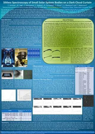
E N D
Slitless Spectroscopy of Small Solar System Bodies on a Dark Cloud CurtainF. Yoshida1, M. Yagi1, Y. Komiyama1, F. Nakata1, H. Furusawa1, T. Ohno2,4, S. Okamura2 and T. Nakamura31National Astronomical observatory of Japan (Mitaka, Tokyo 181-8588 Japan, fumi.yoshida@nao.ac.jp, 2Univesity of Tokyo, 3Teikyo Heisei University, 4MEXT We carried out a slitless spectroscopy using grism filters which was equipped recently to the prime focus camera (Suprime-Cam) of the 8.2 m Subaru telescope. From only one night observation, we could obtain the low dispersion spectra of about 40 small solar system bodies (R<~23 mag). Usually the slit spectroscopic observation of moving object was possible for only the object whose orbit is well known, because of telescope tracking. Therefore it was impossible to obtain the spectra of several moving objects at the same time. However, the slitless spectroscopic observation using grism filters enables to obtain several spectra of moving objects whose orbits are unknown at the same time. Because it is not necessary to put each object into the narrow slit of spectrograph. The slitless spectroscopy by Subaru telescope is a great tool to obtain spectra of very small solar system bodies with an unprecedented efficiency. Introduction : Investigating taxonomic type of small solar system bodies (SSSBs) by spectroscopic observation is really important to estimate material of SSSBs. Moreover, surveying the spatial distribution of each taxonomic type objects would be important to know origin of SSSBs which currently distributed into different groups. Based on the above reasons, the spectroscopic observations of SSSBs have been energetically performed for relatively large SSSBs. Meanwhile, for relatively small SSSBs regarded as collisional fragments, almost no systematic spectroscopic observations have been done, because of their faintness and inaccurate orbits. However, recently the Suprime-Cam brought in new grism filters, then it enabled us to obtain spectra of moving objects up to R~23 mag with 80 min exposures, with low dispersion of 50, with the wavelength coverage of 4500-8600 Å. Since the Suprime-Cam can detect about 100 moving objects (R<~25 mag) in the one FOV (34' x 27'), we obtained the spectra of 40 objects simultaneously. It is unprecedentedly efficient spectroscopic observations for moving objects so far. One of difficulties of slitless spectroscopy (using grisms) is contamination with background objects (faint galaxies of stars). In order to overcome this difficulty, we have had a nice idea that we use a dark cloud of our galaxy as a curtain to avoid contamination from background stars. The curtain worked very well. This poster mentions on our first trial of slitless spectroscopy by using the Subaru telescope and Suprime-Cam grisms. Aim of Science There are two main scientific topics achieved by obtaining the spectra of very small SSSBs. (1) Investigating the origin of meteorites: Fig.9 shows the spectra of different asteroids types which were taken from SMASSII and smoothed to our grism resolution of 50Åin the same range of wavelength coverage. Comparing with those spectra, we are convinced that we are able to determine several asteroid types (S, Q, C, D) with the slitless spectroscopy. Using this classification, we can search for meteorite reservoirs in the main belt. Most of meteorites are classified as ordinary chondrites which have similar spectra with Q-type asteroids. Q-type asteroids are regarded as collisional fragments of S-type, because (1) intermediate spectra between S-type and Q-type have been found in the Near Earth Asteroids (NEAs) group and (2) it has been confirmed by laboratory experiments that space-weathering process varies Q-type spectra to S-type spectra [10]. It is reasonable to assume that Q-type asteroids which are fragments of S-type asteroids and fall on the earth become meteorites. Our question is "where were Q-type asteroids created?" Since collisional probability at the near-Earth region looks not high enough, it is natural to assume that the Q-type came from the main belt through a usual supply route of NEAs. However Q-type is very rare in the main belt. Only two Q-type asteroids were discovered so far [11] in the extremely young asteroid family, Datura family, which was created 450 kyr ago [12]. Regarding the NEAs, Binzel et al. (2004) [13] suggested that Q-type begins to dominate at D<5km. If we can determine asteroid type for smaller asteroids (D<5km) in the main belt, we may find more Q-types there. If there is a Q-type cluster in the main belt, it must be a meteorite reservoir. 27’ 34’ Fig.3 CCD array of Suprim-Cam: 10 CCDs of 2K x 4K FOV: 34’ x 27’ (equivalent to the full moon size) (2) Investigating small Jupiter Trojans:Very recently, Fernandez et al. (2009) [14] found that the median R-band albedo of small JTs (5km<D<24km) is much higher (0.12) than that of large JTs with D>57 km (0.04). This means that there is a possibility that small Trojans show different spectral-type from large Trojans. So far, there is no spectral information of JTs of a few to several tens km in size. We can detect such objects and obtain their spectra with the slitless spectroscopy. Fig.9 Spectra of known asteroids in SMASSII [15].S, Q, D, and C types are plotted from left to the right normalized at 5500Å. Spectra are taken from BB02 and B04, smoothed with the grism resolution, and resampled by 50Å in 4500Å-8600Å. The difference of S and Q is seen in the slope at >7500Å Fig.1 8.2m Subaru telescope at Mauna Kea in Hawaii Fig.2 Prime Focus Camera: Suprime-Cam Observations :We observed the ρOph region (centered at RA.16:27:24.2, Dec. -24:25:06 J2000) [9]with theBlue grism (4500-7000Å) and Red grism (6250-8600Å)in a single night on May 26, 2009. For calibrations, we also took B, R, i-bands images at the same night. We observed LDS749B for flux calibration and Landolt stars of SA107 for photometric calibration. For wavelength calibrations, we used QSOs and the absorption line of A-band of stars (7619 Å) for Red grism and the Hel line of LDS749B for Blue grism. We used Dome flat. For orbit determination, we observed the ρOph region in additional two nights, but only for 12 minutes in R band in each night. Detected Moving objects : The idea of using the ρOph as a curtain was proved to work quite well. The faintest objects detected in each exposure have ~ 23 Rmag (AB). The S/N of spectra of such faint objects are ~1.5 in 6-min exp. image of blue grism data, and ~1 in 3-min exp. image of red grism data. A total of 289 SSSBs with R<25 mag were detected in R-band images in this three-night observing run. 99 SSSBs were detected 3 days consecutively. Then, the Minor Planet Center gave the designation number of 85 SSSBs. 16 of them were known asteroids. In addition, we estimated orbits of 198 SSSBs from only their motion because of their short observation arc (one or two nights). 6 moving objects beside the edge of images were lost. The total numbers of detected SSSBs of each of the asteroid groups are as follows. The figures in parentheses are the numbers of objects which we estimated their orbits from just their motions. The spectra of 37 objects with R<23 mag were obtained. We classified the spectra in the table below. Fig.4 Red grism :Two unit grisms 17.0 cm x 7.4 cm x 1.7 cmx 2 (top and bottom) cover theFOV of Suprime‐Cam. This grism frame is inserted inthe optical path like a band‐pass filter. Fig.5 Left: Dark cloud, Right: Subaru Deep field near galactic pole. Green circle show objects (B < 20.5 mag) from UNSO-B1 catalogue. There are fewer objects with B > 20 mag in the dark cloud region than near galactic pole. That's why the dark cloud is suitable for slitless spectroscopy. Fig.6 Left: the apparent magnitude distribution of moving objects detected in this survey. Right: the absolute magnitude distribution of the same moving objects. The X show the cumulative distribution for objects corresponding to D=1- 0.5 km size. The slope of cumulative distribution fitted by a power law distribution is 1.42. This is similar to the slope obtained by Yoshida et al. (1.2-1.3) [1]~[5] and SDSS survey (1.4) for the main belt asteroids. Fig.7 A part of image of the slitless spectroscopy with the Suprime-Cam. One can see the images of stars, MBAs and a TNO and their spectra. Most of the spectra are free from overlapping. The image and spectra of MBAs are elongated along their motion during exposure. Fig. 8 Examples of spectra from grism observations. The upper images are from the blue (top) and red (bottom) grisms. The clump at the left is the 0-th order light and the ticks in the images show 4000, 6000, and 8000 Å, from the left to the right. The lower graphs show the bule and red spectra connected by using the reflectance at 6400‐6800 A. The spectra were normalized at 5500 Å. Green dots with error bars show the photometric point with the B‐, Rc‐, and i‐bands. The small black dotted lines in the graph show appropriate asteroid spectra derived from SMASSII (Fig.9) which give reasonable fit to our observation. Summary : We observed ρOph cloud and detected 289 SSSBs (R<25 mag). We obtained grism spectra of 37 SSSBs (R<23 mag) from a single night observation. We could determine the orbits for 85 objects by using the observational arc of 3 consecutive nights and for 198 objects by just their velocities. Then we divided detected objects into asteroid groups (inner, middle, outer belt, Hilda, Jupiter Trojan and TNO). We classified asteroids into 4 types by their grism spectra. Based on our preliminary results, the middle belt seems to have most variety of asteroid types (S:43%, Q:33%, C:14%, D:10%). Our preliminary analysis so far indicates that there are more Q types in the middle belt than in the inner belt. This might mean that there is one of supply sources of Q type (meteorite) in the middle belt. Motivated by this successful pilot observation in 2009, we performed the same observation again in the ρOph cloud region in 3 nights in 2010 June. Now the data reduction is going on. We are supposed to obtain grism spectra of each object over 3 nights and then expect to obtain spectra for fainter objects. References: [1] Yoshida et al. 2001, PASJ, 53, L13. [2] Yoshida et al. 2003, PASJ, 55, 701. [3] Yoshida and Nakamura 2004, AdSpR, 33, 1543. [4] Yoshida and Nakamura 2005, AJ, 130, 2900. [5] Yoshida and Nakamura 2007, P&SS, 55, 1113. [6] Yoshida and Nakamura 2008, PASJ, 60, 297. [7] Nakamura and Yoshida (2008) PASJ, 60, 293. [8] Strom et al., Science, 2005, 309, 1847. [9] Dobashi et al. (2005) PASJ, 57, S1. [10] Sasaki et al. (2001), Nature, 410, 555. [11] Mothe-Diniz and Nesvorny, 2008, A&A, 486, L9. [12] Nesvorny, et al. 2006, Science, 312, 1490. [13] Binzel et al. (2004) Icarus, 170, 259 (B04). [14] Fernandez et al. 2009, AJ, 138, 240. [15] Bus, S.J. and Binzel, R.P. (2002) Icarus, 158, 146 (BB02)