Download
1 / 28
300 likes | 559 Vues
Networks in Metabolism and Signaling Edda Klipp Humboldt University Berlin Lecture 3 / WS 2007/08 Random Networks: Scale-free Networks. Random Networks: Scale-free Networks. Most “natural” networks do not have a typical degree value, they are free of a characteristic

E N D
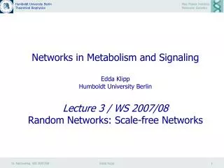
Networks in Metabolism and Signaling Edda Klipp Humboldt University BerlinLecture 3 / WS 2007/08Random Networks: Scale-free Networks
Random Networks: Scale-free Networks Most “natural” networks do not have a typical degree value, they are free of a characteristic “scale”: they are scale-free. Their degree distribution follows a Power law: P(k) ~ k-g Heterogeneity: hubs with high connectivity, many nodes with low connectivity.
Random Networks: Scale-free Networks The probability that a node is highly connected is statistically more significant than in a random graph, the network’s properties often being determined by a relatively small number of highly connected nodes that are known as hubs. Barabási–Albert model of a scale-free network: Growth: Start with small number of nodes (m0) At each time point add a new node with m ≤ m0 links to the network Preferential attachment: Probability for a new edge is where kI is the degree of node I and J is the index denoting the sum over network nodes. The network that is generated by this growth process has a power-law degree distribution that is characterized by the degree exponent g = 3.
Evolution of Scale-free Networks After t time steps network with N = t + m0nodes and m t edges. Continuum theory: ki as continuous real variable, change proportional to P(ki)
Evolution of Scale-free Networks After t time steps network with N = t + m0nodes and m t edges. Continuum theory: ki as continuous real variable, change proportional to P(ki) Degree distribution independent of time t And independent of network size N But proportional to m2
Evolution of Scale-free Networks After t time steps network with N = t + m0nodes and m t edges. Master equation approach: probability p(k,ti,t) that a node i introduced at time ti has degree k at time t. Main idea: Dorogovtsev&Mendes-2001
Scale-free Networks: Clustering coefficient No inherent clustering coefficent C(k)
Scale-free Networks: Average Path Length Shortest path length l: distance between two vertices u and v with unit length edges Fully connected network: Rough estimation for random network: Average number of nearest neighbors: <k> vertices are at distance l or closer total number of vertices
Scale-free Networks: Average Path Length Is obtained by fitting
Scale-free Networks: Error and Attack Tolerance Question: consider arbitrary connected graph of N nodes and assume that a p fraction of edges have been removed. What is the probability of the resulting graph being still connected? Usually: existence of a threshold probability pc. More severe: removal of nodes
Scale-free Networks: Error and Attack Tolerance Node Removal The relative size S(a),(b) and average path length l (c),(d) of the largest cluster in an initially connected network when a fraction f of the nodes are removed. (a),(c) Erdös-Renyi random network with N=10 000 and <k>=4; (b),(d) scale-free network generated by the Barabasi-Albert model with N=10 000 and <k>=4. , random node removal; º, preferential removal of the most connected nodes.
Random Networks: Scale-free Networks Difference to classical random networks: Growth of the network – given number of nodes Preferential attachment – equal probability for all edges Examples: References in www: connections frequently to existing hubs Metabolism: many molecules are involved in only a few (1,2) reactions, others (like ATP or water) in many Wagner/Fell: highly connected molecules are evolutionary “old”
Properties of Scale-Free Networks Small-world – short paths between arbitrary points Robustness – Topological robustness
Watts & Strogatz Model Problem: real networks have short average path length and greater clustering coefficients than classical random graphs Construction: Initially, a regular one dimensional lattice with periodical boundary conditions is present. Each of L vertices has z ≥ 4 nearest neighbors. Then one takes all the edges of the lattice in turn and with probability p rewires to randomly chosen vertices. In such a way, a number of far connections appears. Obviously, when p is small, the situation has to be close to the original regular lattice. For large enough p, the network is similar to the classical random graph.
Watts-Strogatz-Model By definition of Watts and Strogatz, the smallworld networks are those with “small” average shortest path lengths and “large” clustering coecients. <k>remains constant During rewiring
Random Networks: Hierarchical Networks To account for the coexistence of modularity, local clustering and scale-free topology in many real systems it has to be assumed that clusters combine in an iterative manner, generating a hierarchical network. The starting point of this construction is a small cluster of four densely linked nodes. Next, three replicas of this module are generated and the three external nodes of the replicated clusters connected to the central node of the old cluster, which produces a large 16-node module. Three replicas of this 16-node module are then generated and the 16 peripheral nodes connected to the central node of the old module, which produces a new module of 64 nodes….
Random Networks: Hierarchical Networks Clustering coefficent scales with the degree of the nodes
Application to Metabolic Networks Jeong H et al, 2000, Nature
Metabolic Networks: Pathway Lengths E.coli 43 different organisms
Metabolic Networks: Robustness Hubs removed first Random removal M=60 – 8% of substrates
Protein-Protein-Interaction Networks • Yeast proteome • Map of protein-protein interactions • Largest cluster: 78% of all proteins • Red – lethal • Green – non-lethal • Orange – slow-growth • Yellow – unknown • Cut-off: kc=20 • b) Connectivity distribution • c) Fraction of essential proteins with • k links Random removal – no effect Hubs removal – lethal
Protein-Protein-Interaction Networks Random removal – no effect Hubs removal – lethal 93% of proteins have 5 or less links only 21% of them are essential 0.7% of proteins have more than 15 links 62% of them are lethal