Gradient Domain High Dynamic Range Compression
Gradient Domain High Dynamic Range Compression. Raanan Fattal Dani Lischinski Michael Werman. The Dynamic Range Problem. What’s wrong with these images? What would your eye see? How could you put all this information into one image?. Whole Image Solutions. Tone Reproduction Curves

Gradient Domain High Dynamic Range Compression
E N D
Presentation Transcript
Gradient Domain High Dynamic Range Compression Raanan Fattal Dani Lischinski Michael Werman
The Dynamic Range Problem • What’s wrong with these images? • What would your eye see? • How could you put all this information into one image?
Whole Image Solutions • Tone Reproduction Curves • Re-mapping of luminance values • Easy to compute • Suffer from quantization • Examples • Linear scaling • Gamma correction • More sophisticated models…
Ward Larson Model • One of the best total image methods • Based on models of display capabilities and human vision • Still suffers from loss of local contrast • Notice washed-out appearance of the outside area
Local Solutions • Tone Reproduction Operators • Take local context into account • Attempt to solve the local contrast problem • Older Methods • Based on estimating illuminance and reflectance for each part of the image • Suffer from artifacts, dark halos
Low Curvature Image Simplifier • Tumblin and Turk, 1999 • Scale luminance of smoothed image • Add back details • 8 parameters • Computationally intensive
Basic Assumptions • The eye responds more to local intensity differences than global illumination • A HDR image must have some large magnitude gradients • Fine details consist only of smaller magnitude gradients
Basic Method • Take the log of the luminances • Calculate the gradient at each point • Scale the magnitudes of the gradients with a progressive scaling function (Large magnitudes are scaled down more than small magnitudes) • Re-integrate the gradients and invert the log to get the final image
1D Example Original Signal F(x) - Dynamic range: 2415:1
1D Example ln F(x)
1D Example F’(x)
1D Example G(x) = F’(x) after applying the attenuating function
1D Example I(x) = Integrate G(x)
1D Example eI(x) - New dynamic range: 7.5:1
Changes for 2D • Use gradients instead of derivatives • May produce a non-integrable vector field after scaling • Transform scaled vectors into a conservative field whose gradients are closest to G(x)
Attenuation Details • Images contain edges at multiple levels of detail • How do we handle this? • Compute gradients for many different resolutions of the image • The set of different resolution images composes a Gaussian pyramid
Creating the Final Image • How do we recombine the different resolution levels? • Start with coarsest image • Calculate scaling factors • Linearly interpolate those factors for each point in the next image, and multiply with the local scaling factor • Apply the combined factors to the highest resolution image
The Attenuation Function • α = average gradient magnitude for each level times 0.1 • β = adjustable gain (between 0.8 and 0.9)
Performance • On an 1800 MHz Pentium 4: • Computing a 512x384 image takes 1.1 seconds • Computing a 1024x768 image takes 4.5 seconds • LCIS takes 8.5 minutes to compute a 751x1130 image
Examples • Streetlight on a foggy night • Dynamic range 100,000:1
Examples • Stanford Memorial Church • DR 250,000:1
Applications • Enhancing contrast for LDR images • Combining photographs of different exposure levels to enhance detail or stitch together for panoramas • Medical image enhancements
Questions / Credits • Any questions? • All pictures in this presentation are from the original paper