Download
1 / 20
210 likes | 826 Vues
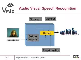
A Multi-Stream Approach to Automatic Audio-Visual Speech Recognition Mark Hasegawa-Johnson Electrical and Computer Engineering. Audio-Visual Speech Recognition. Dual-Stream Model of Speech Perception (Hickok and Poeppel, 2007) ROVER (Recognizer Output Voting for Error Reduction – Fiscus, 1997)

E N D
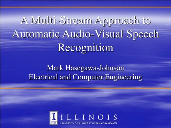
A Multi-Stream Approach to Automatic Audio-Visual Speech RecognitionMark Hasegawa-JohnsonElectrical and Computer Engineering
Audio-Visual Speech Recognition • Dual-Stream Model of Speech Perception (Hickok and Poeppel, 2007) • ROVER (Recognizer Output Voting for Error Reduction – Fiscus, 1997) • Dynamic Bayesian Networks (Zweig, 1998) • Audio-Visual Asynchrony • Coupled HMM (Chu and Huang, 2000) • Articulatory Feature Model • AVSR Results
Dual-Stream Model of Speech Processing (Hickok and Poeppel, 2007, Fig. 1)
… or are there three paths (left and right ventral streams?)(Hickok and Poeppel, 2007, Fig. 2)
ROVER (Recognizer Output Voting for Error Reduction) (Fiscus, 1997) “Left Ventral Stream” “Right Ventral Stream” “Dorsal Stream” First-pass recognizers insert edges into a word lattice “like” “a” “ton of” t1 t2 t3 “tough” t0 “liar” ROVER algorithm: choose edge with the most votes
How to Implement each of the Streams: Dynamic Bayesian Network • Bayesian Network = A Graph in which • Nodes are Random Variables (RVs) • Edges Represent Dependence • Dynamic Bayesian Network = A BN in which • RVs are repeated once per time step • Example: an HMM is a DBN • Most important RV: the “phonestate” variable qt • Typically qtЄ {Phones} x {1,2,3} • Acoustic features xt and video features yt depend on qt
Example: HMM is a DBN wt-1 wt winct-1 winct ft-1 ft qt-1 qt qinct-1 qinct xt-1 yt-1 xt yt Frame t-1 Frame t • qt is the phonestate, e.g., qtЄ { /w/1, /w/2, /w/3, /n/1, /n/2, … } • wt is the word label at time t, for example, wt Є {“one”, “two”, …} • ft is the position of phone qt within word wt: ftЄ {1st, 2nd, 3rd, …} • qinct Є {0,1} specifies whether ft+1=ft or ft+1=ft+1
Example of a Problem DBNs can Solve: Audio-Visual Asynchrony • Audio and Video information are not synchronous • For example: “th” (/q/) in “three” is visible, but not yet audible, because the audio is still silent • Should HMM be in qt=“silence,” or qt=/q/?
A Solution: Two State Variables(Chu and Huang, ICASSP 2000) • Coupled HMM (CHMM): Two parallel HMMs • qt: Audio state (xt: audio observation) • vt: Video state (yt: video observation) • dt=bt-ft: Asynchrony, capped at |dt|<3 wt-1 wt winct-1 winct ft-1 ft qinct-1 qinct qt-1 qt xt-1 xt dt-1 dt bt-1 bt vinct-1 vinct vt-1 vt yt-1 yt Frame t-1 Frame t
word word ind1 ind1 U1 U1 sync1,2 sync1,2 S1 S1 ind2 ind2 U2 U2 sync2,3 sync2,3 S2 S2 ind3 ind3 U3 U3 S3 S3 Asynchrony in Articulatory Phonology(Livescu and Glass, 2004; based on Browman and Goldstein, 1992 etc.) • It’s not really the AUDIO and VIDEO that are ssynchronous… • It is the LIPS, TONGUE, and GLOTTIS that are asynchronous
Asynchrony in Articulatory Phonology • It’s not really the AUDIO and VIDEO that are ssynchronous… • It is the LIPS, TONGUE, and GLOTTIS that are asynchronous “three,” dictionary form Tongue Dental /q/ Retroflex /r/ Palatal /i/ Glottis Silent Unvoiced Voiced time “three,” casual speech Tongue Dental /q/ Retroflex /r/ Palatal /i/ Glottis Silent Unvoiced Voiced
Asynchrony in Articulatory Phonology • Same mechanism represents pronunciation variability: • “Seven:” /vәn/→ /vn/ if tongue closes before lips open • “Eight:” /et/ → /e?/ if glottis closes before tongue tip closes “seven,” dictionary form: /sevәn/ Lips Fricative /v/ Tongue Fricative /s/ Wide /e/ Closed /n/ Neutral /ә/ time “seven,” casual speech: /sevn/ Lips Fricative /v/ Tongue Fricative /s/ Wide /e/ Closed /n/ Neutral /ә/ time
An Articulatory Feature Model(Hasegawa-Johnson, Livescu, Lal and Saenko, ICPhS 2007) • There is no “phonestate” variable. Instead, we use a vector qt→[lt,tt,gt] • Lipstate variable lt • Tonguestate variable tt • Glotstate variable gt wt-1 wt winct-1 winct lt-1 lt linct-1 linct lt-1 lt dt-1 dt tt-1 tt tinct-1 tinct tt-1 tt et-1 et gt-1 gt ginct-1 ginct gt-1 gt
Experimental Test (Hasegawa-Johnson, Livescu, Lal and Saenko, ICPhS 2007) • Training and test data: CUAVE corpus • Patterson, Gurbuz, Turfecki and Gowdy, ICASSP 2002 • 169 utterances used, 10 digits each, silence between words • Recorded without Audio or Video noise (studio lighting; silent bkgd) • Audio prepared by Kate Saenko at MIT • NOISEX speech babble added at various SNRs • MFCC+d+dd feature vectors, 10ms frames • Video prepared by Amar Subramanya at UW • Feature vector = DCT of lip rectangle • Upsampled from 33ms frames to 10ms frames • Experimental Condition: Train-Test Mismatch • Training on clean data • Audio/video weights tuned on noise-specific dev sets • Language model: uniform (all words equal probability), constrained to have the right number of words per utterance
Experimental Questions(Hasegawa-Johnson, Livescu, Lal and Saenko, ICPhS 2007) • Does Video reduce word error rate? • Does Audio-Video Asynchrony reduce word error rate? • Should asynchrony be represented as • Audio-Video Asynchrony (CHMM), or • Lips-Tongue-Glottis Asynchrony (AFM) • Is it better to use only CHMM, only AFM, or a combination of both methods?
Results, part 1: Should we use video?Answer: YES. Audio-Visual WER < Single-stream WER
Results, part 2: Are Audio and Video be asynchronous?Answer: YES. Async WER < Sync WER.
Results, part 3: Should we use CHMM or AFM?Answer: DOESN’T MATTER! WERs are equal.
Results, part 4: Should we combine systems?Answer: YES. Best is AFM+CH1+CH2 ROVER
Conclusions • Video reduces WER in train-test mismatch conditions • Audio and video are asynchronous (CHMM) • Possible models of asynchrony: • “Ventral stream:” CHMM maps acoustics to phones, as directly as possible • “Dorsal stream:” AFM computes the posterior probabilities of lip, tongue, and glottis gesture combinations; words are a by-product • Best result: combine both representations