Download
1 / 21
230 likes | 417 Vues
The Geography of Biological Diversity. Species-Area Curves. S = species richness A = size of the sampling plot (eg. m 2 ) c and z are fitting parameters. c is higher in biodiverse areas z is higher where species richness rises quickly with area.

E N D
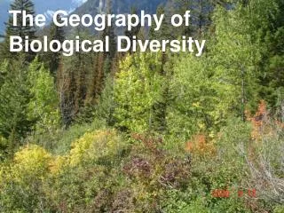
The Geography of Biological Diversity
Species-Area Curves S = species richness A = size of the sampling plot (eg. m2) c and z are fitting parameters • c is higher in biodiverse areas • z is higher where species • richness rises quickly with area
Why does species number increase with area? • Small sampling plots miss some species that happen not to be there • Such plots may only represent a small subset of all microhabitats Does it make sense to plot species richness within political units? Shrub Biodiversity in the United States
Species area curves tell us nothing about species evenness Are species found with similar frequency, or are some dominant while most are rare? The Shannon Index A mathematical index of diversity that accounts for both species richness and evenness The Shannon Index is generally expressed as
Calculating the Shannon Index SUM eH’ Species evenness A mathematical index of diversity that accounts for both species richness and evenness
Proportional Distribution of Known Species • Known Knowns • There are about 1.7 • million known species • Known unknowns • Other species exist • Unknown unknowns • The total number is • highly uncertain (4 to 20 • million species may exist) • ‘Unknown’ knowns • Indigenous knowledge of • other species in remote • areas • In addition to species • diversity, we are also • learning more about • genetic diversity within • species World Conservation Monitoring Centre (1992)
MAMMALS • The number of species • increases toward the • equator, with exceptions • for some groups of • organisms • Peninsulas have lower • diversity than adjacent • mainland areas, • especially toward the • tip of the peninsula • Species diversity • tends to decrease with • elevation, except in • arid regions TREES BIRDS Notice the reverse gradient of species diversity in Florida and the Yucatan
Why is biodiversity higher in the tropics? • Historical theories of biodiversity • Assumes that patterns of biodiversity are not in • true equilibrium with modern environmental conditions • Repeated glacial events of the Pleistocene caused mass • extinctions at higher latitudes • Evolution is far too slow to rebuild species richness between • events • Stability-time HypothesisLong periods of environmental stability enhance species • richness (time for speciation to occur) • Problem: much of tropical rainforest may have been taken • over by savanna during glaciation events
Evidence of Historical Theory of Biodiversity Two lakes: Lake Baikal (Russia) and Great Slave Lake (Canada) Both are deep, cold water bodies Lake Baikal was never glaciated Great Slave Lake appeared 10,000 years ago (postglacially) Great Slave Lake 4 species of deep water benthic invertebrates Lake Baikal 580 species of deep water benthic invertebrates, many endemic
II. Equilibrium theories of biodiversity • Larger resource gradients in • warm, moist areas (1) • More specialized niches can • be occupied in high resource • areas (2) • If interspecific competition is a factor, high resource availability may allow more specialist niches to be sustained (3a) • Areas of high biodiversity occur where there is high • resource availability: relaxation of competitive pressure enables more generalist species to co-occur (3b) LARGERRESOURCEGRADIENTS MORESPECIALIZEDNICHES LESS COMPETITIONFOR ABUNDANTRESOURCES (MORE OVERLAP)
Habitat Diversity as a Control on Biodiversity • Complex topography • Hydrological gradients • Variable solar radiation and microclimate • Mountains cause climatic variation • Greater surface area • Vegetation structure • Each stratum differs • in terms of vegetation • structure, plant • composition and • microclimate • Problems: (i) It is largely the higher diversity in vegetation • that causes the stratification. There are exceptions (eg. high • mammal diversity in savanna)
IV. Environmental Stability as a Control on Biodiversity • Stable climate enables species to become finely-adapted and • to develop the most efficient forms of behaviour to take • advantage of resources without trade-offs • Species then become increasingly specialized and occupy • more and more niches • High latitude species may be forced into certain elements of • generalization (eg. temperature tolerance) • Competition • Adaptation to interspecific competition instead of climate • VI. Predation • High numbers of predators and parasites keep prey • populations low, thereby avoiding competitive exclusion
VII. Productivity • Autotrophs of high productivity environments produce • more energy that can be used to support a larger number • of species at higher trophic levels
Island Biogeography Species richness tends to increase with potential habitat area ISLANDS LAKES DESERT SPRINGS MOUNTAINS Each are ‘insular’ See lab notes for more details
Less unoccupied niche space Higher chance of extinction (lower resource availability, more competition)