Download
1 / 11
110 likes | 270 Vues
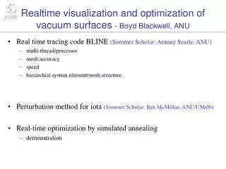
Realtime visualization and optimization of vacuum surfaces - Boyd Blackwell, ANU. Real time tracing code BLINE (Summer Scholar: Antony Searle, ANU) multi-thread/processor mesh accuracy speed hierarchial system element/mesh structure

E N D
Realtime visualization and optimization of vacuum surfaces - Boyd Blackwell, ANU • Real time tracing code BLINE (Summer Scholar: Antony Searle, ANU) • multi-thread/processor • mesh accuracy • speed • hierarchial system element/mesh structure • Perturbation method for iota (Summer Scholar: Ben McMillan, ANU/UMelb) • Real-time optimization by simulated annealing • demonstration
Minimal Confinement Geometries • Simplest possible geometries with closed surfaces that resemble real geometries, for testing codes • fast direct evaluation, exact • iota ~ 1 • aspect ratio ~ 5-10 • highly 3D • enclose no conductors • “triator” • 4 simple elements (finite filaments) • iota ~ 0.6, bean shaped, (similar to Tom Todds?) • “1 element” toroidal helix • slow evaluation
Mesh Interpolation • cubic tri-spline on regular rectangular meshes • copy of mesh in neighbourood stored to better fit in CPU cache • derivatives stored only in local mesh (4 point eval from main mesh) • mesh hierarchy underneath the hierarchy of magnetic macro-elements • e.g. H-1 has 3 meshes for main field, but one coarse mesh for VF coils • allows quick configuration exploration by varying currents (linear combination I1M1 + I2M2 + I3M3) • mesh filled on demand and/or in background • (see also Gourdon code, Zacharov’s code (Hermite polynomials)) H-1 TFC VF 3 ea. 32×128×32
Mesh Convergence • Meshes of 10-50MByte are adequate even near edge • distance to nearest conductorrecorded in each cell, automatically revert to direct calculation if too close. 5th order or better in x
Multi-processing • windows threads (posix under linux) (MISD) • needs semaphore system (e.g. no tracing while loading a new mesh) • multi-threaded code runs fine on single processor • some priority tuning useful on single processor • initial scheme • tracing thread, display thread and mesh-filling threads • large caches on Intel machines favour each thread working in distant memory locations • multi-threading object oriented coding
Perturbation Calculation of iota B B0 • Find a nearby rational surface by iteration ~middle order • say ~ 30 circuits • Store B and derivatives along this closed path • For each variation in the perturbing winding, integrate x B/B0 whereB is the perturbing field and B0 the original field • (Alternatively integrate cpt of B in surface, normalized to B0 and the puncture spacing at that point ~ Boozer )
Accuracy of / I • Check / I by ultra highaccuracy (1e-7) directcalculation of • correction for area changecan be significant Perturbation result: 0.315 cf 0.304
Machine Optimization of iota • Minimization by steepest descent (but multi-variate) • Simulated annealing • virtual temperature T • accept a new configuration even if slightly worse (up to T) • “heat” to explore new configurations • “cool” to home in on optimum • Annealing more tolerant of occasional anomalies in goodness function, e.g. local minima or discontinuities (resonances)
“Reinvent” helical conductor in flexible heliac • Constrain conductor to lie inside a torus, N=3 • (actually end-point and middle point fixed) • Seek maximum transform for length current • Result is very close to the flexible heliac
R>Rmin constraint “sawtooth coil” • Constrain conductor to lie on a cylinder, N=3 • Seek maximum transform near the axis of a heliac per unit length current • Reproduces approximate “sawtooth coil”
Conclusions and Future Work • Very useful for following particles out of machine (so far, not a drift calculation) • Very quick (50k/sec) configuration evaluation for varying current ratios in existing coil system (e.g. H-1 flexibility studies) • Fast evaluation (10k/sec) of new winding (“simple”) in arbitrarily complex existing configuration • Iota perturbation calculation works, and is fast. • Well calculation implemented, but not debugged • Possibly extend to island width as in Rieman & Boozer 1983 • optimization principle demonstrated • “standard results” recovered • real time operation possibility of human guidance during optimization Develop/find “Meta-Language” for description of symmetries and constraints