Groundwater Extraction Impact Study for Water Resources Management

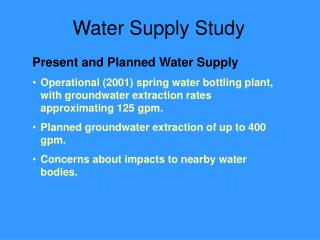
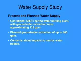
1. Water Supply Study • Present and Planned Water Supply • Operational (2001) spring water bottling plant, with groundwater extraction rates approximating 125 gpm. • Planned groundwater extraction of up to 400 gpm. • Concerns about impacts to nearby water bodies.

2. Critical Prediction Calculate changes in Surface-Water Flows, Wetland and Lake Levels from Constant Production of 400 gpm

3. Regional Model Design Selected Code MODFLOW2000 Model Summary 4 layers Conductivity zones derived from regional/local geologic studies Variable recharge derived from published regression analysis Study Area

4. Local Model Area Groundwater Flow Pumping Center Impoundment Spring Outfall Stream

5. Shortcomings in Problem Formulation • Modeling Tool – Use of River Package • Inability to realistically represent changes in streams, wetlands, and lakes. • Inability to explicitly represent the impoundment-overflow

6. Stream Impoundment Culvert Discharge Stream

7. Revised Problem Formulation • Digitized stream intersections and topo maps to assign MODFLOW Drain/River - revised during calibration. • Impoundment and nearby lakes represented with Lake Package (Merritt and Konikow, 2000); outflow from impoundment explicitly modeled. • Four wetlands with standing water modeled with Lake Package to explicitly simulate wetland water levels. • Stream simulated using MODFLOW Drain Package plus Impoundment outflow. • Regional river comprises down gradient drainage center.

8. Model Calibration • Calibration Strategy • Steady-state calibration to water levels in 48 wells, baseflow in five creeks, and lake levels in five lakes. • Transient calibration to drawdowns from long-term (72 hour) pumping test - one dozen wells with time-series drawdown data • Prior information used to establish total transmissivity as ‘soft’ information during steady-state calibration • Approx. 40 parameters – step-wise reduction using tied/untied parameters as calibration progressed • PEST used in parallel across four 1.8GHz processors

9. PEST Pre-Post Processing • Advantages over GUI or ‘prompt’ Execution • Ability to assess progress with every run • Ability to re-parameterize (tie, hold, transform, scale, prior, regularize) model without ‘rebuild’ • Ability to alter run type with one (or two) quick Control File modifications – Forward run, Estimation, Regularization, and Prediction

10. program fluxes c Read output from MF2K Lak package modified by Mark Kuhl, to sum c baseflows over target reaches and write to single file for use c as PEST targets. c General declarations parameter(ncol=243,nrow=164,nlay=4) implicit double precision (c,d,r,g,s,m, b) dimension riv(:,:), drn(:,:), iriv_rch(:,:) , idrn_rch(:,:) integer kper, kstp, jj, i, j, k, idrn_rch, iriv_rch, nriv, idum c Files produced by MKUHL's MODFLOW Package character*20 drnfile, rivfile character*23 lakfile c Output file from this program for PEST character*12 pestout c Specific Target Names c 1: COLE_CREEK: Drain Reach 1 c 2: GILBERT_CREEK: Drain Reach 2, River Reach 2 c 3: DEAD_STREAM: Drain Reach 3 c 4: BURDON_CREEK: River Reach 3 c 5: MUSKEGON_RIVER: River Reach 4 + SUMMED COMPONENTS allocatable riv, drn, idrn_rch, iriv_rch allocate(riv(ncol,nrow),drn(ncol,nrow), idrn_rch(ncol,nrow), + iriv_rch(ncol,nrow)) drnfile='drain_cell_flows.dat' rivfile='river_cell_flows.dat' lakfile='lake_flow_and_level.dat' pestout='pestout.dat' idrn_rch=0 iriv_rch=0 c======================================================================= c MAIN PROGRAM START c======================================================================= c Read drain flows: KPER, KSTP ,R, C, Q (L^3/T) Open(1,file=drnfile) Read(1,*) Do jj=1,20000 c Use drntemp to account for multiple reaches in one cell drntemp=0. read(1,1,end=991) kper, kstp, i, j, drntemp drn(j,i) = drn(j,i)+drntemp End do 991 Close(1) c Read river flows: KPER, KSTP ,R, C, Q (L^3/T) Open(1,file=rivfile) Read(1,*) Do jj=1,20000 c Use rivtemp to account for multiple reaches in one cell rivtemp=0. read(1,1,end=992) kper, kstp, i, j, rivtemp riv(j,i) = riv(j,i) + rivtemp End do 992 Close(1) c Read Osprey Lake outflows, and stages for the five simulated lakes Open(1,file=lakfile) Read(1,*) sprey_out, sL1, sL2 Close(1) c======================================================================= c 1: COLE CREEK - Comprises drains ONLY: SG-103 c======================================================================= c Drain flows within COL-ROW range COLE_CREEK = 0. do i=1,nrow do j=1,ncol if (i.ge.21.and.i.le.121) then if (j.ge.16.and.j.le.144) then COLE_CREEK = COLE_CREEK + drn(j,i) idrn_rch(j,i) = 1 endif endif end do end do c Subtract flows which accumulate and go northwards at divide COLE_NORTH = 0. do i=1,nrow do j=1,ncol if (i.ge.32.and.i.le.47) then if (j.ge.42.and.j.le.49) then COLE_NORTH = COLE_NORTH + drn(j,i) idrn_rch(j,i) = 0 endif endif end do end do COLE_CREEK = COLE_CREEK - COLE_NORTH c======================================================================= c 2: GILBERT_CREEK - Comprises drains and rivers: SG-101 c======================================================================= c Drain flows within COL-ROW range GILBERT_DRAIN = 0. do i=1,nrow do j=1,ncol if (i.ge.16.and.i.le.96) then if (j.ge.166.and.j.le.211) then GILBERT_DRAIN = GILBERT_DRAIN + drn(j,i) idrn_rch(j,i) = 2 endif endif end do end do c River flows upgradient of drain delineation GILBERT_RIVER = 0. do i=1,nrow do j=1,ncol if (i.ge.4.and.i.le.15) then if (j.ge.16.and.j.le.210) then GILBERT_RIVER = GILBERT_RIVER + riv(j,i) iriv_rch(j,i) = 2 endif endif end do end do GILBERT_CREEK = GILBERT_DRAIN + GILBERT_RIVER write(*,*) GILBERT_DRAIN, GILBERT_RIVER c======================================================================= c 3: DEAD_STREAM - Comprises drains and Osprey Lake Outflow: SG-102 c======================================================================= c Drain flows within COL-ROW range DEAD_STREAM = 0. do i=1,nrow do j=1,ncol if (i.ge.97.and.i.le.113) then if (j.ge.175.and.j.le.204) then DEAD_STREAM = DEAD_STREAM + drn(j,i) idrn_rch(j,i) = 3 endif endif end do end do c Osprey Lake outflows: use NEGATIVE of Sprey_out as this is +ve DEAD_STREAM = DEAD_STREAM + (-SPREY_OUT) c======================================================================= c 4: BURDON_CREEK - Comprises rivers only: SG-104 c======================================================================= c River flows within COL-ROW range BURDON_CREEK = 0. do i=1,nrow do j=1,ncol if (i.ge.92.and.i.le.126) then if (j.ge.11.and.j.le.53) then BURDON_CREEK = BURDON_CREEK + riv(j,i) iriv_rch(j,i) = 3 endif endif end do end do c======================================================================= c 5: MUSKEGON_RIVER - All drainage contributing to tri-lakes: SG-105 c======================================================================= c Begin by summing all the components calculated above MUSKEGON_RIVER = 0. MUSKEGON_RIVER = COLE_CREEK + GILBERT_CREEK + DEAD_STREAM + + BURDON_CREEK Write(*,*) 'MUSKEGON TRIBS :', MUSKEGON_RIVER c Now account for river cells representing the main lakes, etc. do i=1,nrow do j=1,ncol if (i.ge.89.and.i.le.125) then if (j.ge.54.and.j.le.213) then MUSKEGON_RIVER = MUSKEGON_RIVER + riv(j,i) C if (riv(j,i).ne.0) then C write(*,*) j,i,riv(j,i) C end if iriv_rch(j,i) = 4 endif endif end do end do Write(*,*) 'MUSKEGON TRIBS + WEST RIVERS:', MUSKEGON_RIVER do i=1,nrow do j=1,ncol if (i.ge.126.and.i.le.128) then if (j.ge.197.and.j.le.211) then MUSKEGON_RIVER = MUSKEGON_RIVER + riv(j,i) iriv_rch(j,i) = 4 endif endif end do end do Write(*,*) 'MUSKEGON TRIBS + MID RIVERS :', MUSKEGON_RIVER do i=1,nrow do j=1,ncol if (i.ge.129.and.i.le.129) then if (j.ge.209.and.j.le.211) then MUSKEGON_RIVER = MUSKEGON_RIVER + riv(j,i) iriv_rch(j,i) = 4 endif endif end do end do Write(*,*) 'MUSKEGON TRIBS + ALL BODIES :', MUSKEGON_RIVER c======================================================================= c Write target data to single file for PEST c======================================================================= COLE_CREEK = (LOG10(-COLE_CREEK)) GILBERT_CREEK = (LOG10(-GILBERT_CREEK)) DEAD_STREAM = (LOG10(-DEAD_STREAM)) BURDON_CREEK = (LOG10(-BURDON_CREEK)) MUSKEGON_RIVER= (LOG10(-MUSKEGON_RIVER)) if (sprey_out.gt.0.) then Sprey_out = (LOG10(Sprey_out)) else sprey_out = 0. End if Open(1,file=pestout) Write(1,'(a30)') 'FLUX TARGET MODELED' Write(1,'(a19,e15.7)') 'COLE_CREEK :', COLE_CREEK Write(1,'(a19,e15.7)') 'GILBERT_CREEK :', GILBERT_CREEK Write(1,'(a19,e15.7)') 'DEAD_STREAM :', DEAD_STREAM Write(1,'(a19,e15.7)') 'BURDON_CREEK :', BURDON_CREEK Write(1,'(a19,e15.7)') 'MUSKEGON_RIVER :', MUSKEGON_RIVER Write(1,'(a19,e15.7)') 'OSPREY LAKE OUTFL :', Sprey_out Write(1,'(a19,e15.7)') 'OSPREY LAKE LEVEL :', sL1 Write(1,'(a19,e15.7)') 'LAKE 2 LEVEL :', sL2 Write(1,'(a19,e15.7)') 'LAKE 3 LEVEL :', sL3 Write(1,'(a19,e15.7)') 'LAKE 4 LEVEL :', sL4 Write(1,'(a19,e15.7)') 'LAKE 5 LEVEL :', sL5 Close(1) Write(*,*) 'GILBERT_CREEK :', GILBERT_CREEK c======================================================================= c Read original MODFLOW DRN and RIV packages, and assign REACHES c======================================================================= c Comment-out the GOTO to re-write packages with reach numbers goto 20 Open(1,file='MICHIGAN_No_Reaches.riv') Open(2,file='Michigan_reaches.riv') c MODFLOW 2000 headers Read(1,*) Read(1,*) Read(1,*) nriv,idum Write(2,'(2I10)') nriv,idum Read(1,*) nriv Write(2,*) nriv c Lay, Row, Col Do n=1,nriv Read(1,*) k,i,j,stage,cond,rbot Write(2,2) k,i,j,stage,cond*10,rbot,iriv_rch(j,i) End do Close(1) Close(2) Open(1,file='MICHIGAN_No_Reaches.drn') Open(2,file='Michigan_reaches.drn') c MODFLOW 2000 headers Read(1,*) Read(1,*) Read(1,*) nriv,idum Write(2,'(2I10)') nriv,idum Read(1,*) nriv Write(2,*) nriv Do n=1,nriv c Lay, Row, Col Read(1,*) k,i,j,rbot,cond Write(2,3) k,i,j,rbot,cond,idrn_rch(j,i) End do Close(1) Close(2) 20 Continue c======================================================================= c FORMAT STATEMENTS c======================================================================= 1 Format(4I11,F21.0) 2 Format(3I10,F10.3,E10.3,F10.3,I10) 3 Format(3I10,F10.3,E10.3,I10) c======================================================================= c END OF PROGRAM c======================================================================= STOP 'Normal Exit' END Batch and Post-Processing Batch File Post-Processor REM File Management del headsave.hds copy mich_fin.hds headsave.hds del mich_fin.hds del mich_fin.ddn del calibration.hds REM Run array multiplers cond_mult rech_mult REM Run custom MF2K Lake Package cust_lak3 <modflowq.in REM get the water level target data targpest REM get the flux target data flux_targets copy mich_fin.hds calibration.hds REM Check for water above land surface wl_above_ls

11. Calibration Results – SS Baseflows Water Levels WL Sum of Squares (PHI) = ~ 115 ft2 Count = 48 wells Mean Residual = - 0.2 ft Mean Absolute Residual = 1.1 ft StDev of the residuals = 1.5 ft Range = 63 ft StDev/Range = ~ 2.25%

12. Calibration Results – Transient Drawdowns

13. Predictive Analysis • Problem Formulation and Execution • Reformulate the PEST calibration control file to estimate the max and min baseflow depletions in stream, while maintaining calibration – i.e. establish the range of uncertainty • Typically the increment added to the calibration objective function (Fmin + d) is about 5% of Fmin. • For our analysis, this was raised by 50%

14. Predictive Analysis • Present and Planned Water Supply • With total planned groundwater extraction of 400 gpm. • Predicted stream depletion at regional river: 400 gpm • Depletion of interest stream: small but measurable* • Changes in wetland water levels: small but measurable* • The calculated upper- and lower-bound estimates of the change in flow at the stream are on the order of five percent (above or below) of the ‘most likely’ estimated change. • *This is consistent with the observation that wetland water levels, and the areal extent of wetlands based on aerial photographs were not significantly affected by the construction of the impoundment .

15. Salient Point(s) • Problem formulation is key to the ‘integrity’ of the predictive analysis – the selected code must be designed to simulate the type of prediction of interest. • The fairly tight bounds on the prediction may also arise from the ability of models to predict changes far better than absolute numbers.