Ray Tracing in GeoComputation
Ray Tracing in GeoComputation. Sanjay Rana Department of Civil and Environmental Engineering University College London s.rana@ucl.ac.uk. Topics Ray Tracing Applications in GIS Implementing Ray Casting within GIS Conclusions. Ray Tracing

Ray Tracing in GeoComputation
E N D
Presentation Transcript
Ray Tracing in GeoComputation Sanjay Rana Department of Civil and Environmental Engineering University College London s.rana@ucl.ac.uk
Topics Ray Tracing Applications in GIS Implementing Ray Casting within GIS Conclusions
Ray Tracing Technique to trace the path of a (light) ray through a scene and calculating the reflection, refraction, and absorption of the ray when it interacts with the objects in the scene. Viewpoint-based Ray Tracing Light-based Ray Tracing
Ray Tracing Originally developed for gamma radiation related experiments. Now mostly used in Computer Graphics for rendering photorealistic scenes. Three spheres that reflect off each other and the floor Transparency and Shadow details
Ray Tracing Two general types of ray tracing principles: 1a. Ray Casting: A simple approach to identify objects visible from the viewpoint e.g. “Are two locations visible to each other?” Or “What is the nearest object to the viewpoint”? 1b. Radiosity, Photon Mapping etc. types: Based on the entire path a light ray travels after reflection, refraction, and absorption e.g. computation of soft shadows and transparency. Several orders more complicated than Ray Casting.
1a. Ray Casting Visibility Polygon or Isovist Pseudo Code: (i) Cast a ray starting at the viewpoint, pointing to a direction or the desired target. (ii) Intersect ray with each objects along the ray path. (iii) Collect nearest intersection. (iv) For Line of Sight (LOS) test, check if the nearest intersection is on the desired target. OR Repeat steps (i)-(iii) for entire 360o view for creating a visibility polygonor isovist.
1b. Radiosity, Photon mapping etc. types • Pseudo Code: • Create a ray at the viewpoint or light source, pointing in any direction. • Intersect ray with an object. • Use a rendering equation or some wave propagation model to evaluate what happens to the ray i.e. incident angles, how much reflected, absorbed etc. • Repeat steps (i)-(iii) for the reflected/refracted ray and keep repeating (iv) for several runs. • Repeat steps (i)-(iv) for many many rays till a satisfactory solution (in case of computer graphics, photorealism) has been achieved.
Ray Tracing The objective of the talk is to show you some quite unique applications of this computer graphics technique in GeoComputation. For detailed information on ray tracing, please refer to numerous literature on ray tracing in books, papers.
2. Applications in GIS 2a.Urban visibility analysis Morphometry of open spaces Wayfinding models 2b.Wireless reception modelling 2c.Geometrical analysis of shapes Medial Axis Transform
2a. Urban visibility analysis Intellectually challenging study of indoor and outdoor built environments with applications ranging from accessibility evaluation, pedestrian behaviour modelling, visual surveillance, and visual impact assessment (aesthetics). Architecture surrounding urban open spaces is geometrically quite complex for analysis. Void or open space between architecture is a sort of mirror of the architecture and can be easily characterised.
2a.1 Morphometry of open spaces Based on generalising the open space with a dense mesh of viewpoints (i.e. rasterisation) and computing an isovist for each of the viewpoints by Ray Casting. The shape of an isovist (i.e. a spot in the open space) can be described in terms of several 2D morphological measures . Most commonly derived using 2D building plans and street networks.
2a.1 Morphometry of open spaces • Pseudo code: • Create a dense mesh of viewpoints in the open space. • Cast a ray from a viewpoint in a direction and collect the nearest intersection point. • Repeat step (ii) in very fine angular intervals (≤0.1o) over 360o. • Join up all intersection points to form the isovist and compute shape measures. • Repeat steps (ii)-(iv) for all viewpoints.
2a.1 Morphometry of open spaces r d Area: The amount of visible space. Radial (r) and Diametric (d)length: The length of line of sight or ray from the viewpoint. Circularity: Level of resemblance of the isovist polygon to a circle; Circularity = π.r2 / [area of isovist], r = average radial length.
2a.1 Morphometry of open spaces Dense Mesh of 4298 viewpoints Isovist Area High Tate Britain Gallery, London Low Circularity Longest Diametric Length
2a.2 Wayfinding models Enormous amount of multi-disciplinary research on the kind of clues in the open space, people use in deciding their path in a shopping mall, roads, hospitals and so on. Some simple clues include: the direction with the most amount of area visible (following the light) and the direction along the furthest visible point (following the radials). Some research also on Random Walk. Empirical studies have been done which found weak to reasonable level of correlation between the simulated directions of movement and actual path people take.
2a.2 Wayfinding model A very crude exploratory walk Pseudo Code: Generate a dense mesh of viewpoints in the open space. Compute the direction of longest radial and longest radial length (LRL) for each viewpoint. Place the observer(s) of the walk anywhere. Find the viewpoint with the longest radial in the neighbourhood of the observer(s). Take the MRL direction of this neighbour and move the observer one step in that direction. Repeat steps (iv) – (v).
5-60 60-150 150-185 185-275 275-350 N Direction of Longest Radials based on 5o ray intervals 12 steps of six observers exploring the polygon based on the LRL
2b. Wireless Reception modelling Planning of Radio and Cell Phone antennas coverage involves modelling the transmission of radio and micro waves within the urban infrastructure. It is basically a radiosity type ray tracing except with different equations and generally a location-allocation requirement. At present, wireless reception modelling is carried out with third party plug-ins, which use finite element numerical mathematics. There will be a rise in demand for this application due to the increasing focus on embedding Wi-Fi networks (e.g. for seamless VOIP services) and cell phone technology in cities.
2b. Screenshots of Wireless System Engineering (WiSE) software tool developed by Bell Laboratories Signal Strength Plot Ray Traces in WISE See also: Wagen and Rizk (2003). Radiowave propagation, building databases, and GIS: anything in common? A radio engineer's viewpoint, E&P-B, 30(5), 767-787.
2c. Geometrical Analysis of Shapes Understanding the shape of geographical representations (e.g. contours, polygons) is useful in certain spatial operations (e.g. when converting contours to DEMs, finding out the road centre lines). At present, most solutions are based on differential geometry, utilising the variations in the coordinates of the shape outlines. Some of the morphometric measures derived from ray tracing are also useful and in some cases (e.g. 3D shapes) will be even more easier to compute.
2c.1 Medial Axis Transform (MAT) Linking the centres of circles and spheres, which touch the boundary of a shape at least twice. MAT is a popular technique to identify the “skeleton” of shapes in many disciplines ranging from medical imaging to computer graphics hence also called skeletonization. In GeoComputation, it has been used in detecting feature lines in contours during triangulation to avoid flat triangles (Gold and Dakowicz 2001). Contour Medial Axis Flat Triangles Correct shape after adding medial axis
2c.1 Medial Axis Transform (MAT) A trivial way to do MAT is to perform the Distance Transform, which involves discretising the shape and computing the shortest distance from each cell/voxel to the boundary. The shortest distance to the boundary is in fact same as the shortest radial length derived by ray tracing. The cells at local extremum are skeletal points and the medial axis coincides with the ridge line. A landscape type plot of shortest radial length. Note that the ridges coincide with the medial axis.
3. Implementing Ray Casting within GIS The run time of basic Ray Casting is O(mn), where m is the average number of intersection tests around a viewpoint and n is the number of viewpoints. Radiosity type ray tracing will require several orders more computation time. Roughly, the number of intersections depends upon the number of obstacles and number of rays from the viewpoint (>> 3600). The software architecture in most of the existing off-the-shelf GI systems leads to extremely long computation time because of the following reasons: Scripts are interpreted and not compiled into machine language. More efficient data structures such as graphs and trees are not available to the developer.
3. Implementing Ray Casting within GIS Computation time of ray casting can be speeded up by several techniques e.g. by converting the scene into Binary Space Partitioning Tree structure (BSP Tree). In short, BSP Tree divides the space by planes (l1, l2,l3, l4) into a set of convex polygons. From BSP tree we can find out where the viewer is placed (a very simple point-in-polygon query) and the objects in that convex polygon. So we do not have to perform intersection tests with all polygons. l2 l1 l4 l3
3. Implementing Ray Casting within GIS Demonstration of Isovist Analyst
4. Conclusions Ray Tracing is a technique for tracing the path of rays in a 2D or 3D Scene. Ray Tracing can be used in several types of GeoComputation e.g. urban viewshed, wireless reception modelling and geometrical analysis of shapes. The simpler version of Ray Tracing, namely Ray Casting will certainly be a very useful function in existing GI Systems. It could “simply” be the “missing” 2D analogy of the terrain viewshed function e.g. the Visibility function in ArcObjects. The computation requirements are high but could be substantially reduced with heuristics.
Acknowledgements Discussions and software support: Yiorgos Chrysanthou for the BSP code Frank Warmerdam for Shapefile libraries. Images: http://en.wikipedia.org/wiki/Ray_tracing http://aec.cadalyst.com/aec/article/articleDetail.jsp?id=155714 Conroy and Dalton (1999) for the Tate Gallery outline. http://www.bell-labs.com/org/wireless/wisext.html for WISE images http://www.voronoi.com/pdfs/2000-2003/Terrain_Modelling_from_Contours.pdf for MAT and Terrain modelling figures. Isovist Analyst can be downloaded for free from: http://www.ucl.ac.uk/~ucessan/software/isovist-analyst.htm This presentation would soon be available online at: http://eprints.ucl.ac.uk/perl/search/advanced?&creators=rana