Download
1 / 26
260 likes | 281 Vues
This study in Nepal's Terai region explores LiDAR data calibration for satellite models, forest type mapping, and emission level estimates. By integrating satellite imagery, LiDAR technology, and field data, accurate carbon stock assessments and emission reduction targets are determined in forest conservation programs. The research showcases the feasibility and cost-effectiveness of LiDAR applications, emphasizing the importance of ongoing monitoring using satellite images and LiDAR-derived models.

E N D
Use of Lidar for estimating Reference Emission Level in Nepal S.K. GautamDFRS, Nepal
Introduction: Study Area • Nepal’s ER-Program covers 12 jurisdictional Terai districts out of 75 districts of the country; • Total area under the ER-Program is 2.3 million ha (about 15% of the country); • About 52% of the ER-Program area (1.18 million ha) is under different types of forest cover. • The area islinked with eleven trans-boundary protected areas across Nepal and India and is home to flagship species like tigers, rhinos, Asiatic wild elephants, and many other endangered species. • Total population of the ER-Program area is 7.35 million and constitute about 27% of total population (2011 population census)
Introduction: LAMP • Samples (5%) of LiDAR data to • calibrate satellite models; • Reference field sample plots to calibrate/validate LiDAR models; • Landsat satellite imagery forwall-to-wall biomass map.
LiDAR block design • Stratificationfrom a Landsat-based forest classification map. • Weight calculated for every block as a product of the importance of the forest types and the inverse of the forest types area. • The forest classification was used as a priori information to calculate weighting function for random block and systematic plot design. • 5 km x 10 km systematic grid over the study area where ew is the expert weight and A is the area
LiDAR block design Forest type map with forest type weights. The larger weights are with brighter tones in gray-scale. Black = zero weight (non-forest).
Basics of a REDD+ RL • The basic math is: • Activity Data (ha change/year) × Emissions Factors (tCO2/ha) = tCO2/year • Activity data is be based on satellite information (past) or assumptions (future) • Emissions factors are based on field measurements and allometric equations
Activity Data • Defines forest/non-forest for 1999 inception date of RL with 1998 Topographic basemaps • Utilizes satellite analysis for 1999, 2001, 2006, 2009 and 2011 to delineate structural classes of intact, degraded and deforested • Bases classification on fractional image indexes (i.e., % vegetation) and temporal analysis drawing on work by leader in the field Carlos Souza of Brazil • Develops land cover change matrix by tracking changes between the different structural classes between 4 time-periods
Emissions Factors • DFRS, FRA, Arbonaut and WWF collaborate in collection of LiDAR data covering 5% of TAL program area in 2011 • Field plots collected in 2011 (738 calibration plots) and 2013 (46 validation plots) • Uses allometric equations of Sharma and Pukkala (1990) to estimate biomass for ground plots (same equations used by FRA)
Emissions Factors • Model to correlate LiDAR-based above-ground biomass estimates for each forest condition (intact, deforested, degraded and regeneration) and forest type (Sal, Sal mixed, Other mixed and Riverine) • IPCC default values used to calculate mean carbon density for regeneration and below-ground carbon based on biomass estimates
Results: Historical CO2 emissions Average annual net CO2 emissions (tCO2e) in TAL between 1999 and 2011.
Accuracy assessment • a) Comparison to independent field plots • b) Leave-one-out validation LAMP model (Landsat) LiDAR model Estimated biomass (t/ha) R2 = 0.52 R2 = 0.92 Field-measured biomass (t/ha)
Research and Development: Difference in AGB between 1999-2011
Costs and Future Monitoring • The cost of this project is USD 0.28/ha • Our experience shows that 1-2% LiDAR coverage is sufficient for this integrated approach • But LiDAR is needed only once • Subsequent monitoring is based on new satellite images to which the LAMP models are applied
Decision Tree and Definition of Forest for Terai Arc Landscape
Forest types and conditions map • Four major forest types: 1) Sal forest, 2) Sal dominated mixed forest, 3) other than Sal dominated forest (i.e. “other forest”) and 4) Riverine. • The four forest types were overlaid on the forest structural map (Joshi et al. 2003) to generate forest types and conditions maps for each time period. • The study assumed forest types do not change from one type to another type (i.e., from Sal forest to mixed forest or riverine forest or vice versa) in 10-20 years;