Download
1 / 25
250 likes | 363 Vues
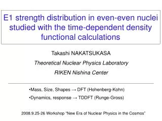
E1 strength distribution in even-even nuclei studied with the time-dependent density functional calculations. Takashi NAKATSUKASA Theoretical Nuclear Physics Laboratory RIKEN Nishina Center. Mass, Size, Shapes → DFT (Hohenberg-Kohn) Dynamics, response → TDDFT (Runge-Gross).

E N D
E1 strength distribution in even-even nuclei studied with the time-dependent density functional calculations Takashi NAKATSUKASA Theoretical Nuclear Physics Laboratory RIKEN Nishina Center • Mass, Size, Shapes → DFT (Hohenberg-Kohn) • Dynamics, response → TDDFT (Runge-Gross) 2008.9.25-26 Workshop “New Era of Nuclear Physics in the Cosmos”
Basic equations Time-dep. Schroedinger eq. Time-dep. Kohn-Sham eq. dx/dt = Ax Energy resolution ΔE〜ћ/T All energies Boundary Condition Approximate boundary condition Easy for complex systems Basic equations Time-indep. Schroedinger eq. Static Kohn-Sham eq. Ax=ax(Eigenvalue problem) Ax=b (Linear equation) Energy resolution ΔE〜0 A single energy point Boundary condition Exact scattering boundary condition is possible Difficult for complex systems Energy Domain Time Domain
How to incorporate scattering boundary conditions ? • It is automatic in real time ! • Absorbing boundary condition γ A neutron in the continuum n
Potential scattering problem For spherically symmetric potential Phase shift
Time-dependent picture Scattering wave Time-dependent scattering wave (Initial wave packet) (Propagation) Projection on E :
Boundary Condition Absorbing boundary condition (ABC) Absorb all outgoing waves outside the interacting region How is this justified? Finite time period up to T Time evolution can stop when all the outgoing waves are absorbed.
s-wave nuclear potential absorbing potential
3D lattice space calculationSkyrme-TDDFT Mostly the functional is local in density →Appropriate for coordinate-space representation Kinetic energy, current densities, etc. are estimated with the finite difference method
Skyrme TDDFT in real space Time-dependent Kohn-Sham equation 3D space is discretized in lattice Single-particle orbital: N: Number of particles Mr: Number of mesh points Mt: Number of time slices y [ fm ] Spatial mesh size is about 1 fm. Time step is about 0.2 fm/c Nakatsukasa, Yabana, Phys. Rev. C71 (2005) 024301 X [ fm ]
Real-time calculation of response functions • Weak instantaneous external perturbation • Calculate time evolution of • Fourier transform to energy domain ω [ MeV ]
Nuclear photo-absorptioncross section(IV-GDR) 4He Cross section [ Mb ] Skyrme functional with the SGII parameter set Γ=1 MeV 0 100 50 Ex [ MeV ]
12C 14C 10 20 30 40 Ex [ MeV ] 10 20 30 40 Ex [ MeV ]
18O 16O Prolate 10 30 20 40 Ex [ MeV ]
26Mg 24Mg Triaxial Prolate 10 20 30 40 10 20 30 40 Ex [ MeV ] Ex [ MeV ]
28Si 30Si Oblate Oblate 10 20 30 40 Ex [ MeV ] 10 20 30 40 Ex [ MeV ]
32S 34S Prolate Oblate 10 20 30 40 10 20 30 40 Ex [ MeV ] Ex [ MeV ]
40Ar Oblate 40 20 30 10 Ex [ MeV ]
44Ca Prolate 48Ca 40Ca 10 20 30 Ex [ MeV ] 10 20 30 40 Ex [ MeV ] 10 20 30 40 Ex [ MeV ]
Electric dipole strengths Z SkM* Rbox= 15 fm G = 1 MeV Numerical calculations by T.Inakura (Univ. of Tsukuba) N
Peak splitting by deformation 3D H.O. model Bohr-Mottelson, text book.
Centroid energy of IVGDR O Fe Cr C He Ne Mg Be Si Si Ar Ca Ti
Low-lying strengths S Mg Si Ar Be Ne Ca C O Ti He Cr Fe Low-energy strengths quickly rise up beyond N=14, 28
Summary Small-amplitude TDDFT with the continuum Fully self-consistent Skyrme continuum RPA for deformed nuclei Photoabsorption cross section for light nuclei Qualitatively OK, but peak is slightly low, high energy tail is too low For heavy nuclei, the agreement is better. Theoretical Nuclear Data Tables including nuclei far away from the stability line → Nuclear structure information, and a variety of applications; astrophysics, nuclear power, etc.