Chapter 3 Hubs, Bridges and Switches
730 likes | 868 Vues
Chapter 3 Hubs, Bridges and Switches. Interconnecting LANs. Q: Why not just one big LAN? Limited amount of supportable traffic: on single LAN, all stations must share bandwidth Ethernet: limited length: 802.3 specifies maximum cable length

Chapter 3 Hubs, Bridges and Switches
E N D
Presentation Transcript
Lecture 3 Chapter 3Hubs, Bridges and Switches
Lecture 3 Interconnecting LANs Q: Why not just one big LAN? • Limited amount of supportable traffic: on single LAN, all stations must share bandwidth • Ethernet: limited length: 802.3 specifies maximum cable length • Ethernet: large “collision domain” (can collide with many stations) • collision domain: set of stations such that simultaneous transmission of any two of them will generate a collision • Token Ring: token passing delay per station: 802.5 limits number of stations per LAN:
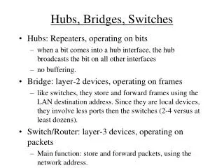
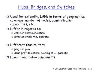
Lecture 3 Hubs • Physical Layer devices: essentially multi-leg repeaters operating at bit levels: repeat bits received on one interface to all other interfaces • Hubs can be arranged in a hierarchy (or multi-tier design), with backbone hub at its top
Lecture 3 Hubs (more) • Each connected LAN referred to as LAN segment • Hubs do not isolate collision domains: node may collide with any node residing at any segment in LAN • Hub Advantages: • simple, inexpensive device • Multi-tier provides graceful degradation: portions of the LAN continue to operate if one hub malfunctions • extends maximum distance between node pairs (100m per Hub)
Lecture 3 Hub limitations • single collision domain results in no increase in max throughput • multi-tier throughput capacity same as single segment throughput • individual LAN restrictions pose limits on number of nodes in same collision domain and on total allowed geographical coverage • cannot connect different Ethernet types (e.g., 10BaseT and 100baseT) Qn: Why?
Lecture 3 Bridges • Link Layer devices: forward Ethernet frames selectively: • learn where each station is located • examine the header of each frame • forward on the proper link (if known) • if dest. and source on same link, drop frame WHY? • if not known where dest. is, broadcast frame • except on originating link, of course • also called Layer 2 switches
Lecture 3 Bridges • Bridge isolates collisiondomains • buffers frame • then forwards it, if needed, using CSMA/CD • A broadcast frame is forwarded on all interfaces (except the incoming one) • thus broadcast frames propagate across bridges • A set of segments connected by bridges and hubs is called a broadcast domain
Lecture 3 Bridges (more) • Bridge advantages: • Isolates collision domains resulting in higher total throughput capacity, and does not limit the number of nodes nor geographical coverage • Can connect different type Ethernet since it is a store and forward device (e.g. 10 & 100BaseT) • Transparent: no need for any change to hosts LAN adapters (invisible to them)
Lecture 3 Backbone Bridge
Lecture 3 Interconnection Without Backbone • Not recommended for two reasons: - single point of failure at Computer Science hub - all traffic between EE and SE must path over CS segment
Lecture 3 Bridges: frame filtering, forwarding • bridges filter packets • same-LAN -segment frames not forwarded onto other LAN segments • forwarding: • how to know on which LAN segment to forward frame?
Lecture 3 Bridge Filtering • bridges learn which hosts can be reached through which interfaces: maintain filtering tables • when frame received, bridge “learns” location of sender: incoming LAN segment • records sender location in filtering table • filtering table entry: • (Node MAC Address, Bridge Interface, Time Stamp) • stale entries in Filtering Table dropped (TTL can be 60 minutes)
Lecture 3 Bridge Operation pseudocode Init: set filtering table to void Case: frame arrives on port P, src MAC , dest MAC /* Table Update stage */ if not listed, or mapped to port not equal P then add mapping P with expiration time else update expiration time /* if listing fits */ /* Frame Forwarding stage */ look up in filtering table: listing “ Q” /* if listed */ if not listed, forward on all ports except P /* “flood */ else,ifQ= P , drop the frame /* WHY ? */ otherwise,forward the frame on port Q only
Lecture 3 Bridge Learning: example Suppose C sends frame to D and D replies back with frame to C • C sends frame, bridge has no info about D, so floods to both LANs 2 and 3 • bridge notes that C is on port 1 • frame ignored on upper LAN • frame received by D
Lecture 3 Bridge Learning: example C 1 • D generates reply to C, sends it • bridge sees frame from D • bridge notes that D is on interface 2 • bridge knows C on interface 1, so selectively forwards frame out via interface 1 only
Lecture 3 B 2 2 A , 1 A , 1 2 2 1 1 A What will happen with loops?Incorrect learning Frame sent from A to B Problems: (1) frame loops infinitely (2) unstable filtering tables
Lecture 3 Loop-free: tree C B A message from Awill mark A’s location A
Lecture 3 Loop-free: tree C B A: A message from Awill mark A’s location A
Lecture 3 Loop-free: tree A: C B A: A message from Awill mark A’s location A
Lecture 3 Loop-free: tree A: A: A: C B A: A: A message from Awill mark A’s location A
Lecture 3 Loop-free: tree A: A: A: C B A: A: A message from Awill mark A’s location A
Lecture 3 Loop-free: tree A: A: A: C B A: A: A message from Awill mark A’s location So a message toA will go by marks… A
Lecture 3 Disabled Bridges-Spanning Tree • for increased reliability, it is desirable to have redundant, alternative paths from source to dest • this causes cycles - bridges may multiply and forward frame forever • solution: organize bridges in a spanning tree and disable all ports not belonging to the tree
Lecture 3 Introducing Spanning Tree • Objective: Find tree spanning all LAN segments • each bridge transmits on a single port • each LAN transmits on a single bridge • Bridges run the Spanning Tree Protocol • Use a distributed algorithm • Objective: select what ports should actively forward frames, and which ports should accept frames • Bridges communicate using special configuration messages (BPDUs) to perform this selection • BPDU = Bridge Protocol Data Unit • STP standardized in IEEE 802.1D
Lecture 3 Method • Each bridge sends periodically a BPDU to all its neighbors • BPDU contains: • ID of bridge the sender views as root (my_root_ID) • known distance to that root • senders own bridge ID • port ID of the port from which BPDU sent
Lecture 3 Introductory STP In order to help understanding STP we first present it as 3 separate algorithms • How to agree on a root bridge? • How to compute a ST for bridges? • How to compute a ST for LAN segments? Actual STP does all 3 functions in the same iterative process Note: we assume throughout that the network is connected
Lecture 3 1. Choosing a root bridge • Assume • each bridge has a unique identifier (ID) • within a bridge each port has a unique ID • Each bridge remembers smallest bridge ID seen so far (= my_root_ID) • including own ID • Periodically, send my_root_ID to all neighbors (“flooding”) (included in BPDU) • When receiving ID, update if necessary • Qn: Is that enough for universal agreement?
Lecture 3 2. Compute ST given a root Idea: each bridge finds its shortest path to the root generate shortest paths tree Output: At each node, parent pointer and distance to root (parent=bridge leading to root along shortest path) Spanning tree T: A link belongs to T iff it connects some bridge to its parent Qn: Does this idea fully specify an algorithm producing a spanning tree? How: Bellman-Ford algorithm
Lecture 3 Distributed Bellman-Ford Assumption: There is a unique root node s • this was done in Step 1 Idea: Each node, periodically, tells all its neighbors what is its distance from s But how can they tell? • s: easy. dists = 0always! • Another node v: • Bridge calls the neighbor with least distance to root - its “parent” • If bridges tie: choose bridge with lowest ID
Lecture 3 Why does this work? • Suppose all nodes start with distance , and suppose that updates are sent every time unit. 2 1 ID=21 ID=3 E 1 1 1 D 2 C 1 ID=17 A 1 0 0 0 ID=7 G 3 2 0 1 B 0 2 F Means: BPDU Means: link admitted to bridge spanning tree B sees same distance from A and E; A chosen since has smaller ID
Lecture 3 Bellman-Ford: properties • Works for any positive link weights w(u,v): • Works also when the system operates asynchronously. • Works regardless of the initial distances
Lecture 3 Actual STP What is missing so far?: • Can’t discard redundant links, since we need to connect host, not just bridges • Instead can disable redundant bridge ports leading to them • Graph model too simple, since there can be many bridges on one LAN (see next slide) • We need to look at forwarding paths and not just graph paths STP protocol does all the “steps” together: • Selection of root bridge • Evaluation of distance to root and parent bridge • Selection of the active ports and blocked ports
Lecture 3 Exampleof a network L6 L2 L5 B A D C E L1 L3 F L7 L4 Note: LAN L2 connects three bridges, 4 ports
Lecture 3 STP plan Objective: prune given network to render a forwarding tree, i.e: • between any two hosts there is a single forwarding path through the network, no loops possible Method: Classify all ports into three types: • Root ports: one for each bridge • Designated ports: one for each LAN • All other ports are blocked Root and designated ports transfer data frames in both directions. Blocked ports don’t transfer data
Lecture 3 BPDU’s (1) • Each bridge sends BPDUs on all its ports. • Based on received BPDUs, bridge determines: • determines Root • finds own distance/cost to root • classifies of own ports: root/designated/blocked • The BPDU contains bridge’s current view of: • the root bridge of the network • own distance to this root • own ID number • the sending port’s ID number
Lecture 3 BPDUs (2) • A BPDU is computed by a bridge for each of its ports and sent out on that port • it will reach all ports attached to port’s LAN • STP prerequisites • each bridge is given a bridge ID number • The ID number is unique in the network • Each port is given a port ID number • The port ID is unique within its bridge • ID numbers assigned manually or automatically • Each link (LAN) has a positive cost
Lecture 3 BPDU Processing in a bridge (1) • Determine current view of root: this is lowest root ID received, including own bridge ID. • Only BPDUs reporting this root are considered in sequel • Compare all reported distances to root. own distance to root= lowest received distance + + cost of the link to the reporting bridge
Lecture 3 Designated Ports • all BPDUs received on a port are compared, including own message sent on it; • the best message has: • smallest root ID and • smallest distance to that root • if tied, choose the one with lowest bridge ID • if tied, choose lowest port ID • Qn: When does the last tie happen? • If the message sent by the bridge on that port is best, label it a designated port • there is exactly one designated port on each LAN
Lecture 3 Root Ports • now compare the best messages received on all the ports of the bridge, according to the same criteria as above • the port on which best message was received is labeled root port • root bridge has no root port • there is exactly one root port per bridge • only root and designated ports receive and send data. • BPDU’s are sent periodically • even after convergence of algorithm • indicate bridge is active / discover failures
Lecture 3 Summary • after convergence: • all bridges agree which bridge is the root • each LAN has exactly one designated port • frames from LAN enter the bridge on that port on the way to root (upstream) • frames coming from root exit the bridge on that port on the way to remote LANs (downstream) • all bridges on LAN agree who is the designated port • a LAN may have any ≥ 0 number of root ports on it • each bridge has exactly one root port • the port leads through a LAN to the parent bridge • this is the next bridge on a shortest path to root • a bridge may have any ≥ 0 number of designated ports • a bridge with no designated ports blocks also the root port, and so becomes inactive
Lecture 3 Notes • only bridges make decisions, LANs are passive • More discussion of the validity of STP will be given in homework and recitation
Lecture 3 Example Spanning Tree • Protocol operation: • Pick a root • Each bridge picks a root port B8 B3 B5 B7 B2 B1 B6 B4
Lecture 3 Example Spanning Tree B8 root port Spanning Tree: B3 B5 B1 root port B7 B2 B7 B2 B4 B5 B6 B1 Root B8 B3 B6 LANs not connecting bridgesomitted here B4
Lecture 3 Spanning Tree Protocol: Execution (B8,root=B8, dist=0) B8 B3 ignore msg B5 B7 B2 B1 (B1,root=B1,dist=0) (B1,root=B1, dist=0) B6 B4 WHY? (B4, root=B1, dist=1) (B6, Root=B1, dist=1)
Lecture 3 Bridges vs. Routers • both are store-and-forward devices • routers: network layer devices (examine network layer headers) • bridges are link layer devices • routers have routing tables, use routing algorithms, designed for Wide Area addressing • bridges have filtering tables, use filtering, learning & spanning tree algorithms, designed for local area
Lecture 3 Routers vs. Bridges Bridges + and - + bridge operation is simpler, requiring less processing - topologies are restricted with bridges: a spanning tree must be built to avoid cycles (with routers cycles are avoided by the Layer 3 routing algorithm) - bridges do not offer protection from broadcast storms (endless broadcasting by a faulty host will be forwarded by a bridge)
Lecture 3 Routers vs. Bridges Routers + and - + arbitrary topologies can be supported, cycling is limited by TTL counters (and good routing protocols) + provide barrier protection against broadcast storms - require IP address configuration (not plug and play) - require higher processing • bridges do well in small (few hundred hosts) while routers used in large networks (thousands of hosts) and in Internet core
Lecture 3 Ethernet Switches • = a powerful bridge • layer 2 (frame) forwarding, filtering using LAN addresses • Switching: A-to-B and A’-to-B’ with no collisions • large number of interfaces • often: individual hosts, star-connected into switch • Ethernet w. no collisions! • = Switched Ethernet • often: includes L3 function
Lecture 3 Ethernet Switches • cut-through switching: frame forwarded from input to output port without awaiting for assembly of entire frame • slight reduction in latency • allow combinations of shared/dedicated, 10/100/1000 Mbps interfaces
Lecture 3 Ethernet Switches (more) Dedicated Shared