Download
1 / 5
50 likes | 179 Vues
This document demonstrates how the relationship between two variables, ( s ) and ( t ), described by the formula ( s = at^c ), can be analyzed using logarithmic transformations. By applying logarithmic laws, we derive the equation ( log(s) = c log(t) + log(a) ), which resembles the form of a straight line equation. This approach allows us to plot ( log(s) ) against ( log(t) ), facilitating the estimation of the constants ( a ) and ( c ) from the gradient and intercept of the graph. The analysis showcases the linear relationship inherent in the data, with practical applications using Excel for visualization.

E N D
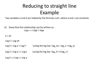
Reducing to straight lineExample Two variables a and b are related by the formula s=atc, where a and c are constants • Show that this relationship can be written as : • Log s = c logt + loga S = atc Log S = Log atc Log S = Log a + Log tc(using the log law logaxy= loga x + logay) Log S = Log a + c Log t (using the log law logaxk= k loga x ) Log S = c Log t + Log a
(ii) Explain why the model can be tested by plotting log y vs log x Compare Log S = c Log t + Log a With the equation of straight line y = m x + c • Log S = c Log t + Log a should give a straight line if s=atc • where : • y = log S • x = log t • m(gradient) = c • c(intercept) = Log a
(iii) Plot log s vs log t and estimate the values of a and c
This looks very linear to me But I need a carefully drawn graph that I can estimate the values of the gradient and intercept from. So I will use Excel
Log s = c logt + loga C (gradient) = Log a S=atc is data relationship where a = 3.98 and c =0.5 Log a = 0.6 a= 100.6 = 3.98 C = 0.5