Download
1 / 46
460 likes | 668 Vues
Linear Network Theory and Sloppy Models. Mark Goldman Center for Neuroscience UC Davis. Outline. Linear network theory essentials Nonlinear networks F itting network models and the “sloppy models” problem. Issue : How do neurons accumulate & store signals in working memory?.

E N D
Linear Network Theory and Sloppy Models Mark Goldman Center for Neuroscience UC Davis
Outline • Linear network theory essentials • Nonlinear networks • Fitting network models and the “sloppy models” problem
Issue: How do neurons accumulate & store signals in working memory? • In many memory & decision-making circuits, neurons • accumulate and/or maintain signals for ~1-10 seconds stimulus accumulation neuronal activity (firing rates) storage (working memory) time Puzzle: • Most neurons intrinsically have brief memories synaptic input Input stimulus r firing rater synapse tneuron ~10-100 ms
“Tuning curve” persistent activity: stores running total of input commands The Oculomotor Neural Integrator Eye velocity coding command neurons excitatory inhibitory Integrator neurons: Firing rate Eye position: Eye position 1 sec time (data from Aksay et al., Nature Neuroscience, 2001; picture of eye from MarinEyes)
Network Architecture Left side neurons Right side neurons 100 100 firing rate firing rate 0 0 Eye Position L R Eye Position L R 4 neuron populations: Excitatory Inhibitory (Aksay et al., 2000) Firing rates: midline Recurrent (dis)inhibition Recurrent excitation background inputs & eye movement commands
tneuron Neuron receiving network positive feedback: Standard Model: Network Positive Feedback 1) Recurrent excitation 2) Recurrent (dis)inhibition (Machens et al., Science, 2005) Command input: Typical isolated single neuron firing rate: time
Many-neuron Patterns of Activity Represent Eye Position saccade Activity of 2 neurons Eye position represented by location along a low dimensional manifold (“line attractor”) (H.S. Seung, D. Lee)
“Chalk talk” section: Linear network theory
Line Attractor Picture of the Neural Integrator Geometrical picture of eigenvectors: r2 No decay along direction of eigenvector with eigenvalue = 1 r1 Decay along direction of eigenvectors with eigenvalue < 1 “Line Attractor” or “Line of Fixed Points”
Next up… • 1) A few comments on linear networks: • Complex eigenvalues • Non-identical time constants • 2) Nonlinear networks & network fitting • 3) The problem of “sloppy models”: how to determine what • was important in one’s model fits
General Case: Unequal t’s, l’s complex Re-write equations as: • Calculate the eigenvectors and eigenvalues. • Eigenvalues have typical form: • The corresponding eigenvector component has dynamics:
Nonlinear networks & Fitting networks to data
Nonlinear Network Model Outputs Wcontra Wipsi Coupled nonlinear equations: Mathematically intractable? Wij = weight of connection from neuron j to neuron i Burst commands & Tonic background inputs Firing rate dynamics of each neuron: Firing rate changes Intrinsic leak same-side excitation opposite-side inhibition Bkgd. input Burst command input
Nonlinear Network Model Outputs Wcontra Wipsi Coupled nonlinear equations: Mathematically intractable? Integrator! Wij = weight of connection from neuron j to neuron i Burst commands & Tonic background inputs Firing rate dynamics of each neuron: Firing rate changes Intrinsic leak same-side excitation opposite-side inhibition Bkgd. input Burst command input For persistent activity: must sum to 0
Fitting the Model Fitting condition for neuron i: Current needed to maintain firing rate r total excitatory current received total inhibitory current received Background input Knowns: -r’s: known at each eye position (tuning curves) -f(r): known from single-neuron experiments (not shown) Unknowns: -synaptic weights Wij > 0 and external inputs Ti -synaptic nonlinearities sexc(r), sinh(r) Assume form of sexc,inh(r) constrained linear regression for Wij, Ti (data = rates ri at different eye positions)
Fitting the Model Fitting condition for neuron i: Current needed to maintain firing rate r total excitatory current received total inhibitory current received Background input Combine recurrent inputs into 1 term: …the form of a standard regression problem!
Fitting the Model Fitting condition for neuron i: Current needed to maintain firing rate r total excitatory current received total inhibitory current received Background input Combine recurrent inputs into 1 term:
Fitting the Model Fitting condition for neuron i: Current needed to maintain firing rate r total excitatory current received total inhibitory current received Background input General time-varying problem (assume t known):
Model Integrates its Inputs and Reproduces the Tuning Curves of Every Neuron Example model neuron voltage trace: Network integrates its inputs …and all neurons precisely match tuning curve data Firing rate (Hz) Time (sec) gray: raw firing rate (black: smoothed rate) green: perfect integral solid lines: experimental tuning curves boxes: model rates (& variability)
…But Many Very Different Networks Give Near-Perfect Model Performance Local excitation Global excitation Circuits with very different connectivity… left exc. left inh. right exc. right inh. left inh. left exc. right exc. right inh. …but nearly identical performance: right side left side
“Sloppy” Models (Models with poorly constrained parameters)
Motivation: “Sloppy” Behavior in Identified Neurons Puzzle: Highly variable data from different instances of a crustacean bursting neuron with highly stereotypical output: Golowaschet al., J. Neurophys., 2002
“Sloppy” Behavior in a Single-Neuron Bursting Model Model neuron 1: Models with 3 spikes per burst (other colors: different #’s spikes/burst) 1000 time (ms) Model neuron 2: time (ms) Goldman et al., J. Neurosci., 2001
Sensitivity Analysis: Which features of the connectivity are most critical? Cost function curvature is described by “Hessian” matrix of 2nd derivatives: Cost function surface: cost C W2 W1 Insensitive direction (low curvature) Sensitive direction (high curvature) diagonal elements: sensitivity to varying a single parameter off-diagonal elements: interactions (Reference: see the work of J.P. Sethna group)
Sensitivity Analysis: Which features of the connectivity are most critical? Cost function curvature is described by “Hessian” matrix of 2nd derivatives: Cost function surface: diagonal elements: sensitivity to varying a single parameter off-diagonal elements: interactions between pairs of parameter eigenvectors/eigenvalues: identify patterns of weight changes to which network is most sensitive cost C W2 W1 Insensitive direction (low curvature) Sensitive direction (high curvature) (Reference: see the work of J.P. Sethna group)
Sensitive & Insensitive Directions in Connectivity Matrix Sensitive directions (of model-fitting cost function) Insensitive Eigenvector 1: make all connections more excitatory Eigenvector 2: weaken excitation & inhibition Eigenvector 3: vary low vs. high threshold neurons Eigenvector 10: Offsetting changes in weights more exc. less inh. less inh. less exc. perturb perturb perturb perturb right side avg. Fisher et al., Neuron, 2013
Diversity of Solutions: Example Circuits Differing Only in Insensitive Components Two circuits with different connectivity… …differ only in their insensitive components Differences between circuits along each component log(difference) -5 -10 …but near-identical performance… right side left side
Exercises: • 1) Symmetric mutual inhibitory/self-excitatory network • 2) Sensitivity analysis of the autapse: • sketch the model sloppy & sensitive directions in (w, t) • assuming experimental data is an exponential decay
Extra Slides: Functionally feedforward & non-normal networks
Recent data: “Time cells” observed in rat hippocampal recordings during delayed-comparison task MacDonald et al., Neuron, 2011: feedforward progression (Goldman, Neuron, 2009) (See also similar data during spatial navigation memory tasks by Pastalkova et al. 2008; Harvey et al. 2012)
Neuronal firing rates Time (sec) Summed output Time (sec) Response of Individual Neurons in Line Attractor Networks All neurons exhibit similar slow decay: Due to strong coupling that mediates positive feedback Problem: Does not reproduce the heterogeneity in neuronal activity seen experimentally! Problem 2: To generate stable activity for 2 seconds (+/- 5%) requires 10-second long exponential decay
Feedforward Networks Can Integrate! (Goldman, Neuron, 2009) Simplest example: Chain of neuron clusters that successively filter an input
Integral of input! (up to duration ~Nt) (can prove this works analytically) Feedforward Networks Can Integrate! (Goldman, Neuron, 2009) Simplest example: Chain of neuron clusters that successively filter an input
Generalization to Coupled Networks: Feedforward transitions between patterns of activity Recurrent (coupled) network Map each neuron to a combination of neurons by applying a coordinate rotation matrix R (Schur decomposition) Feedforward network Connectivity matrix Wij: Geometric picture: (Math of Schur:See Goldman, Neuron,2009; Murphy & Miller, Neuron, 2009; Ganguli et al., PNAS, 2008)
Responses of functionally feedforward networks Functionally feedforward activity patterns… Feedforward network activity patterns & neuronal firing rates Effect of stimulating pattern 1:
Imag(l) persistent mode 1 Real(l) Imag(l) Real(l) no persistent mode??? 1 Math Puzzle: Eigenvalue analysis does not predict long time scale of response! Line attractor networks: Neuronal responses: Eigenvalue spectra: Feedforward networks: (Goldman, Neuron,2009; see also: Murphy & Miller, Neuron 2009; Ganguli & Sompolinsky, PNAS 2008)
Answer to Math Puzzle: Pseudospectralanalysis ( Trefethen & Embree, Spectra & Pseudospectra, 2005) Eigenvalues l: Pseudoeigenvalues le: • Set of all values le that satisfy the inequality:||(W – le1)v|| <e • Govern transient responses • Can differ greatly from eigenvalues when eigenvectors are highly non-orthogonal (nonnormal matrices) • Satisfy equation:(W–l1)v =0 • Govern long-time asymptotic behavior Black dots: eigenvalues; Surrounding contours: colors give boundaries of set of pseudoeigenvals., for different values of e (from Supplement to Goldman, Neuron, 2009)
Imag(l) persistent mode 1 Real(l) Imag(l) Real(l) no persistent mode??? 1 Answer to Math Puzzle: Pseudo-eigenvalues Normal networks: Neuronal responses Eigenvalues Feedforward networks:
Imag(l) persistent mode 1 Real(l) Imag(l) transiently acts like persistent mode Real(l) Answer to Math Puzzle: Pseudo-eigenvalues Normal networks: Neuronal responses Eigenvalues Feedforward networks: Pseudoeigenvals 1 0 -1 1 (Goldman, Neuron,2009)
Practical program for approaching equations coupled through a term Mx • Step 1: Find the eigenvalues and eigenvectors of M. • Step 2: Decompose x into its eigenvector components • Step 3: Stretch/scale each eigenvalue component • Step 4: (solve for c and) transform back to original coordinates. eig(M) in MATLAB
Practical program for approaching equations coupled through a term Mx • Step 1: Find the eigenvalues and eigenvectors of M. • Step 2: Decompose x into its eigenvector components • Step 3: Stretch/scale each eigenvalue component • Step 4: (solve for c and) transform back to original coordinates.
Practical program for approaching equations coupled through a term Mx • Step 1: Find the eigenvalues and eigenvectors of M. • Step 2: Decompose x into its eigenvector components • Step 3: Stretch/scale each eigenvalue component • Step 4: (solve for c and) transform back to original coordinates.
Practical program for approaching equations coupled through a term Mx • Step 1: Find the eigenvalues and eigenvectors of M. • Step 2: Decompose x into its eigenvector components • Step 3: Stretch/scale each eigenvalue component • Step 4: (solve for c and) transform back to original coordinates.
Practical program for approaching equations coupled through a term Mx • Step 1: Find the eigenvalues and eigenvectors of M. • Step 2: Decompose x into its eigenvector components • Step 3: Stretch/scale each eigenvalue component • Step 4: (solve for c and) transform back to original coordinates.
Practical program for approaching equations coupled through a term Mx • Step 1: Find the eigenvalues and eigenvectors of M. • Step 2: Decompose x into its eigenvector components • Step 3: Stretch/scale each eigenvalue component • Step 4: (solve for c and) transform back to original coordinates.