Download
1 / 1
10 likes | 166 Vues

E N D
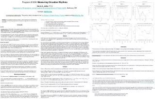
Program #1238: Measuring Circadian RhythmsHarris A. Jaffee, Ph.D. Department of Biostatistics, Johns Hopkins Bloomberg School of Public Health, Baltimore, MD Contact: hj@jhu.eduCommercial relationship: The author was a recipient of an Investigator Initiated Studies Program award from Merck & Co., Inc. Abstract: A new approach to diurnal variation is taken through the time-development of circadian IOP, producing alternatives to the diurnal-range which are more aware of fluctuation. (Fundamental Theorem, continued) • 1. The union of the Ij is disjoint away from the extrema and equals [min(p), max(p)]. • 2. range(p) = max(p)-min(p) is the sum of the Rj. • 3. +(z) is constant on each Oj, say equal to mj. • 4. V(p) may be written as Σ mj*Rj, with each mj ≥1. • 5. V(p) ≥ range(p), with equality if and only if min(p) and max(p) are the only extrema. • The mj are seen as multiplicities, and V is a range-with-multiplicity. • Dynamical interpretation of the positive variation: • Form the differences si = ti+1-ti, and the ratios qi = di/si, which are the slopes of segments of the Jordan polygon, i.e. average rates-of-change of p. V=V(p) may be written Σall i L(qi) * si, where L(q)=0 for q≤0, and L(q)=q otherwise. • Methods • Unlike the diurnal mean which benefits from linearity, the example of R suggests that no measure of DV will be assessable (say in aggregate) from an aggregate diurnal curve, but instead must always be assessed case-by-case (and then, say, averaged). • For a measure of DV to be complete, so that cases may be compared, it must be based on 24-hour c-data, produced from observed diurnal data by diurnalization according to its "scope". The case of multiple days is described above; for a partial day, the replication step by itself produces the only 24-hour pattern possible given the data. Otherwise, let (t0, p0) and (tN, pN) be the first and last data-points, with tN = t0+24-e (e fairly small) and pN = p0-E. To the extent that E is non-zero, these data cannot represent any persisting pattern. If P is the average of p0 and pN, a guess at the implied pattern is made by replacing these two data-points with virtual data points, (t0-e/2, P) and (tN+e/2, P). (A slightly better candidate for P might be the average of the pseudo-data values at t0-e/2 and tN+e/2 determined by linear extrapolation using the 2nd and 2nd-to-last data-points, respectively.) • Given c-data, compute the time intervals s (in decimal hrs) between successive c-data points, the differences d of successive c-data values, and the sequence of ratios q = d/s. Then, the sum Σd>0d (independent of the s) expresses Jordan's positive variation and reflects all fluctuation in the c-data. It is also a range-with-multiplicity, in view of the Fundamental Theorem, so might be called the m-range (M). Writing M as Σq>0q*s, perturbations are suggested such as Σq>0 (eq - 1)*s, which emphasize rate of fluctuation and coincide with M to first-order. This one will be called the x-range (X). Beware that the units of X are complex and involve time. • In order to exercise the calculation of DV, and the effect of a treatment on it, M and X were applied along with R to 24-hour trial data [Konstas-Stewart] of two treatments for OAG, relative to Latanoprost monotherapy. IOP was observed over 24 hours at 4-hour intervals starting at 8am, at baseline and after treatment. For each study eye, treatment, and measure of DV, the DV of that eye's baseline and treatment IOP curves were computed from associated c-data. The difference is the effect of that treatment on the DV of that eye's diurnal IOP, under Latanoprost. • Examples • Figure 1: With patients A and B, the proposed measure M coincides with R. In either measure, B has more DV than A. • Figure 2: R(B) > R(C), but C exhibits an afternoon rise in IOP which is recognized by M, implying the reverse relationship, M(C) > M(B). So in the measure M, C has more DV than B. • Figure 3: Patients C and D have identical R and M. D has a sharper rise in IOP from 12n to 4pm, while C has a sharper rise from 9pm to 7am. X(C) = (e2/4-1)*4 + (e6/10-1)*10 = 10.8, and X(D) = (e3/4-1)*4 + (e5/10-1)*10 = 11.0. In this measure, D has slightly more DV. • The Fundamental Theorem applied to patient C (Fig. 3). The extrema are: 0 < 1 < 3 < 6; R0 = 1, R1 = 2, R2 = 3; m0 = 1, m1 = 2, m2 = 1. V = 2+6 = 8, alternatively m0*R0 + m1*R1 + m2*R2 = 1*1 + 2*2 + 1*3. • Figure 4: Example of diurnalization and resulting c-data, with a large "correction“ to observed data (E=7, Methods). • Figure 5: A small, average reduction in DV of IOP under Bimatoprost relative to Latanoprost. • Figure 6: Average example of diurnal IOP under Dorzolamide relative to Latanoprost, with no effect on DV. • Results • The measures R, M, and X of DV rank cases of diurnal IOP slightly differently. M (resp. X) can also separate the cases with like R (resp. M). For example, M and X can appreciate exfoliation syndrome with an afternoon rise in IOP, while R cannot. • With respect to the measures (R, M, X) of DV applied to the Stewart trial data, relative to Latanoprost, Bimatoprost reduced DV of IOP on average by (1.3, 1.2, 4.3) units, significantly, while Dorzolamide had no significant (average) effect on DV of IOP. • Introduction • Caveats • circadian rhythm is motivated by the example of diurnal intraocular pressure and means the typical daily pattern, possibly manufactured. measuring alludes to a mathematical procedure sought to quantify the relevant, diurnal variation in each instance of a given circadian rhythm. The traditional example is the diurnal range-of-fluctuations. • The clinical procedure (e.g. GAT, Tono-pen, implanted sensor) by which the underlying data are obtained will be assumed here, unspecified. The passage from observed clinical data to "circadian data", or c-data, is via a statistical procedure to be called diurnalization. • Central to the variation of a circadian rhythm is its time derivative as revealed by the c-data. This is a “velocity” (Appendix), albeit abstract. • Clinical precedents • Asrani-Zeimer et al (2000): The diurnal range of fluctuations, for a given eye, was defined as the range (max-min) of the average, over at least 3 consecutive days, of the IOP values for like time-periods, e.g. 6-9 am. Averaging over several days mitigates day-to-day variation, so produces typical values for the time-periods chosen. • The averaging procedure of Asrani-Zeimer is basically the model for diurnalization. It must be enhanced for mathematical “balance”, by replicating the early morning average data value the next morning. This has no effect on the range, and the result is the model for c-data. • Gumus et al (2006), on OAG withexfoliation syndrome (paraphrased): The IOP was highest in the morning, showing a gradual decrease from 8am in the control group, but a second peak at 3pm in 53% of the XS group. All patients had about the same range of fluctuations. • Purpose • Diurnal variation of intraocular pressure is felt to play a major role in the progression of open-angle glaucoma, with the diurnal range (R), perhaps inappropriately applied to a single (or even partial) day of IOP data, taken as the virtual definition. R can only capture overall daily fluctuation. For example, it may be helpless to indicate OAG with XS, even statistically. • The proper meaning of DV would seem to remain obscure, and the goal is a functional formulation. For example, the DV of diurnal IOP should ideally reflect the mechanism of glaucomatous damage. • Diurnal IOP will be viewed through c-data produced by a diurnalization procedure, then explored as a dynamical process, whose time development "carries" all the fluctuation. • Mathematical background • The "total increase" or positive variation, as formulated by Camille Jordan in 1881: • Let pi = p(ti) be the values of a function p at the times t0 < ... < tN, with the difference pi+1-pi denoted di. The positive variation V of p, based on the {ti}, is the sum of those di which are positive. • Definition of circadian process: • Such p is circadian if p(t+24) = p(t) for all t. If also tN = t0+24, then pN = p0, and the N+1 pairs (ti, pi) amount to c-data for p. These points then generate a "polygon" (Jordan) which is the graph of a piecewise-linear function to which p is identified, in approximation, as usual. • Geometric interpretation of the positive variation: • A Fundamental Theorem of Diurnal Variation (adapted from Milnor) • Let p be as above, with extrema min(p) = u0 < ... < uK = max(p). For j<K, let Rj denote the difference uj+1 - uj, i.e. the length of the closed interval Ij = [uj, uj+1], with Oj the “interior” of Ij. Every z in any Oj is a value of p at least twice, and at each occurrence, p is either increasing or decreasing. Write +(z) for the number of times such z occurs while p is increasing. Then: • Conclusions • Two alternatives to the diurnal range are described. The m-range is a strong range, and the x-range a strong m-range. • These alternatives may be better clinical biomarkers than the range, and more useful in glaucoma research, depending on their correlation with progression and visual field loss, which are yet to be determined. • Acknowledgements: The author appreciates the advice and encouragement of Ran Zeimer, William Stewart, and David Guyton. • References • Asrani-Zeimer et al, Large diurnal fluctuations in intraocular pressure are an independent risk factor in patients with glaucoma, J Glaucoma, 2000, Apr, 9(2), p. 134-142 • Brouwer L, Uber Abbildung von Mannigfaltigkeiten, Math Annalen, #71, 1912, p. 97-115 • Gumus et al, Diurnal variation of intraocular pressure and its correlation with retinal nerve fiber analysis in Turkish patients with exfoliation syndrome, Graefe's Arch Clin Exp Ophth, 2006, #244, p. 170-176 • Jordan C, Sur la série de Fourier, Comptes Rendus (Math) Acad. Sci., Paris, #92, 1881, p. 228-230 • Konstas-Stewart et al, 24-hour intraocular pressures with brimonidine purite versus dorzolamide added to latanoprost in primary open-angle glaucoma subjects, Ophthalmology, 2005, Apr;112(4), p. 603-608 • Milnor J, Topology from the Differentiable Viewpoint, University of Virginia Press, 1965 • Appendix • In the Fundamental Theorem, the mj are well-defined and non-zero: • Let -(z) for z in any Oj be the number of times z occurs while p is decreasing, and set #(z) to the sum of +(z) and -(z). This sum is non-zero by continuity (Intermediate Value Theorem) and is also the number of intersections of the graph of p with the horizontal line at height z, so is locally constant. Following any occurrence of z while p is increasing (decreasing), there will eventually be another, similar occurrence by periodicity, hence in between an occurrence of the opposite kind, by continuity again. Thus, -(z) = +(z), and +(z) = #(z)/2, hence +(z) is locally constant. The parity of #(z) is called the mod2 degree of p, and the difference +(z) - -(z) the Brouwer degree [Brouwer, Milnor, mathworld.wolfram.com/MapDegree.html]. Both of these constructs degenerate to zero in this primeval situation. • Action: • Form S = Σq>0 L(q)*s, where L is positive and strictly increasing for q>0, which is phrased more symmetrically as Σall q L(q)*s with L also identically zero for q≤0. (M and X may be expressed this way; R cannot.) Then S is an approximating Riemann sum for the definite integral ∫T L(p'(t))*dt, where p'(t) is the time-derivative of the circadian process p, and T is any 24-hour interval. The integral accumulates, over the day, the occurring values of instantaneous fluctuation, with a prescribed “weighting”. S is an instance of Feynman’s action paradigm [Dirac, Feynman, Brown] with L a particular form of Lagrangian; R is not. • Suggested reading: • Brown L (editor), Feynman's Thesis: A New Approach to Quantum Theory, World Scientific, 2006 • Dirac P, The Lagrangian in Quantum Mechanics, Physik Zeits Sowjetunion, #3, 1933, p. 64- • Feynman R, The Principle of Least Action in Quantum Mechanics, Princeton Thesis, 1942