Morris-Pratt algorithm

1. Morris-Pratt algorithm A linear pattern-matching algorithm, Technical Report 40, University of California, Berkeley, 1970. Advisor: Prof. R. C. T. Lee Reporter: C. S. Ou Morris (Jr) J. H., Pratt V. R.

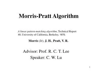
2. Morris-Pratt algorithm We are given a text T and a pattern P to find all occurrences of P in T and perform the comparisons from left to right. n : the length of T m : the length of P Example

3. Rule 1: The Partial Window Rule This rule means that instead of a complete window whose is equal to the size of the pattern, we may use a prefix of a complete window to match the prefix of a prefix of the complete pattern. A complete window T P How do we get the partial window?

4. The basic principle of MP Algorithm is still step by step comparison. Initially, the length of the partial window is 1. Initially, we compare T(1) with P(1). If T(1) ≠P(1), we move The pattern one step towards the right. Example

5. If T(1)=P(1), we extend the partial window until a mismatching is found. Example

6. Suppose the following condition occurs, should we move pattern P only one step towards the right? The answer is no in this case as we may use Rule 2, the suffix of T to prefix of P rule. j i+j-1 j+m-1 1 n T b i m 1 P a Example

7. Rule 2: The Suffix of T to Prefix of P Rule For a window to have any chance to match a pattern, in some way, there must be a suffix of the window which is equal to a prefix of the pattern. T P

8. The Implication of Rule 2: Find the longest suffix v of the window which is equal to some prefix of P. Skip the pattern as follows: T v P v P v

9. Now, we know that a prefix U of T is equal to a prefix U of P. Thus, instead of finding the longest suffix of T equal to a prefix of P, We may simply find the longest suffix of U of P which is equal to a prefix of P. T U b P U a v Example

10. Example In this case, we can see the longest suffix of U which is equal to a prefix of P is CA. Thus, we may apply Rule 2 to move P as follows:

11. The MP Algorithm Assume that we have already found the largest prefix of T which is equal to a prefix of P. t U b p U a

12. The MP Algorithm Skip the pattern by using Rule 1 and Rule 2. T v b P a v v c T v b P c v Given a prefix U of T which is equal to a prefix of P, how do we know the longest Suffix of U which is equal to some prefix of U? We do this by pre-processing.

13. Preprocessing phase for x > 1 and The prefix function Let f(j), 2 ≤j≤m, for P( j) can be written as follows: MP algorithm uses j – g(j) – 1 to decide the distance that pattern P aligns in text T. Example prefix function 1 2 3 4 5 6 7 8 9 10 11 12 13 0 0 0 1 0 1 2 3 4 2 3 4 -1 0 0 0 1 0 1 2 3 4 2 3 4 1 1 2 3 3 5 5 5 5 5 8 8 8 j f(j) g(j) j - g(j)

14. Example prefix function 1 2 3 4 5 6 7 8 9 10 11 12 13 0 0 0 1 j f(j) j = 1 →f(1) = 0 j = 2 →P2 = ‘T’≠ Pf 1(2-1)+1=P1=‘A’ →f(2)=0 j = 3 → P3 = ‘C’≠ Pf 1(3-1)+1=P1=‘A’ →f(3)=0 j = 4 →P4 = ‘A’= Pf 1(4-1)+1=P1=‘A’ →f(4)=0+1=1

15. Example prefix function 1 2 3 4 5 6 7 8 9 10 11 12 13 0 0 0 1 0 1 2 3 4 j f(j) j = 5 →P5 = ‘C’≠ Pf 1(5-1)+1=P1+1=‘T’ →f(5)=0 j = 6 → P6 = ‘A’= Pf 1(6-1)+1=P1=‘A’ →f(6)=0+1=1 j = 7 → P7 = ‘T’= Pf 1(7-1)+1=P1+1=‘T’ →f(7)=1+1=2 j = 8 → P8 = ‘C’= Pf 1(8-1)+1=P2+1=‘C’ →f(8)=2+1=3 j = 9 → P9 = ‘A’= Pf 1(9-1)+1=P3+1=‘A’ →f(9)=3+1=4

16. Example prefix function 1 2 3 4 5 6 7 8 9 10 11 12 13 0 0 0 1 0 1 2 3 4 2 3 4 j f(j) We have found that f(9) = 4. We now check whether P(10)=P(5) . The answer is no. Does this mean that we should set f(9) to be 0? No. j = 10 →P10 = ‘T’≠ Pf 2(10-1)+1=Pf (4)+1=P1+1=P2=‘T’ →f(10)=1+1=2 j = 11 → P11 = ‘C’= Pf 1(11-1)+1=P2+1=‘C’ →f(11)=2+1=3 j = 12 → P12 = ‘A’= Pf 1(12-1)+1=P3+1=‘T’ →f(12)=3+1=4

17. Then, after a shift, the comparisons can resume between characters c = P(f(i )) and T( i +j) = b without missing any occurrence of P in T, and avoiding a backtrack on the text. i+j-1 j+m-1 1 n T u b i m 1 P v u a P Example v c a

18. Example 1 2 3 4 5 6 7 8 9 10 11 12 13 1 1 2 2 2 2 2 7 8 9 10 10 10 prefix function j Shift by 1 j - g(j)-1

19. Example 1 2 3 4 5 6 7 8 9 10 11 12 13 1 1 2 2 2 2 2 7 8 9 10 10 10 prefix function j Shift by 2 j - g(j)-1

20. Example 1 2 3 4 5 6 7 8 9 10 11 12 13 1 1 2 2 2 2 2 7 8 9 10 10 10 prefix function j Shift by 1 j - g(j)-1

21. Example 1 2 3 4 5 6 7 8 9 10 11 12 13 1 1 2 2 2 2 2 7 8 9 10 10 10 prefix function j Shift by 1 j - g(j)-1

22. Example 1 2 3 4 5 6 7 8 9 10 11 12 13 1 1 2 2 2 2 2 7 8 9 10 10 10 prefix function j Shift by 1 j - g(j)-1

23. Example 1 2 3 4 5 6 7 8 9 10 11 12 13 1 1 2 2 2 2 2 7 8 9 10 10 10 prefix function j Shift by 1 j - g(j)-1

24. Example MATCH 1 2 3 4 5 6 7 8 9 10 11 12 13 1 1 2 2 2 2 2 7 8 9 10 10 10 Shift by 10 prefix function j j - g(j)-1

25. Time Complexity preprocessing phase in O(m) space and time complexity searching phase in O(n+m) time complexity

26. References AHO, A.V., HOPCROFT, J.E., ULLMAN, J.D., 1974, The design and analysis of computer algorithms, 2nd Edition, Chapter 9, pp. 317--361, Addison-Wesley Publishing Company. BEAUQUIER, D., BERSTEL, J., CHRÉTIENNE, P., 1992, Éléments d'algorithmique, Chapter 10, pp 337-377, Masson, Paris. CROCHEMORE, M., 1997. Off-line serial exact string searching, in Pattern Matching Algorithms, ed. A. Apostolico and Z. Galil, Chapter 1, pp 1-53, Oxford University Press. HANCART, C., 1992, Une analyse en moyenne de l'algorithme de Morris et Pratt et de ses raffinements, in Théorie des Automates et Applications, Actes des 2e Journées Franco-Belges, D. Krob ed., Rouen, France, 1991, PUR 176, Rouen, France, 99-110. HANCART, C., 1993. Analyse exacte et en moyenne d'algorithmes de recherche d'un motif dans un texte, Ph. D. Thesis, University Paris 7, France. MORRIS (Jr) J.H., PRATT V.R., 1970, A linear pattern-matching algorithm, Technical Report 40, University of California, Berkeley.

27. Thanks for your attention.