Simplex
Simplex. Topics to be covered Introduction to simplex method Flow chart Computational procedure of simplex method Examples. Introduction to Simplex Method


Simplex
E N D
Presentation Transcript
Topics to be covered • Introduction to simplex method • Flow chart • Computational procedure of simplex method • Examples
Introduction to Simplex Method It has not been possible to obtain the graphical solution of more than two variables. In such cases, a simplex method is used which was developed by G. Dantzig in 1947. The simplex method provides a systematic algorithm which consists of moving from one basic feasible solution to another in a prescribed manner so that the value of the objective function is improved.
The simplex algorithm is an step by step procedure for solving LP problems. It consists of: (i) Having a trial basic feasible solutions to constraint equations. (ii) Testing whether it is an optimal solution. (iii) Improving the first trial solution by a set of rules and repeating the process till an optimum solution is obtained In simplex method, One of the non-basic variables at one iteration becomes basic at the following iteration, and it is called an entering variable. One of the basic variables at one iteration becomes non-basic at the following iteration, and is called a departing variable. Back
Back Find the initial basic feasible solution Put the LPP in standard form Construct the starting simplex method Update the new simplex table so obtained Compute ∆j=Zj-Cj=CBXj-cj and examine? Find key element and obtain the new solution by matrix transformation Solution under test is optimal. Stop No Is any ∆j<0 ? Select the row corresponding to min ratio to find the vector leaving the basic B Find the vector Xk entering the basisBsothat ∆k=min∆j Corresponding to any j, are all the elements of entering vector Xk<=0 Solution is unbounded. Stop Solution can be improved. Compute the ratio (XB/XK,XK>0) Yes No
Computational procedure of simplex method Step 1: If the problem is one of minimization, convert it to a maximization problem by considering –z, instead of z, use the min z=-max (-z) Step 2: We checkup all bi’s for non-negativity. If some of the bi’s are negative, multiply the corresponding constraints through by -1 in order to ensure all bi>=0 Step 3: We change the inequalities to equation by adding slack and surplus variable, if necessary. Step 4: We now construct the starting simplex table. From this table, basic feasible solution is obtained. Step 5: We obtain the values of ∆j=Zj-Cj=CBXj-cj and examine the values of ∆j.
There will be three exhaustive possibilities: (i) All ∆j>=0. In this cases, the basic feasible solution under test will be optimal. (ii) Some ∆j<0 and for at least one of the corresponding xj all xrj<=0. In this case , solution will be unbounded. (iii) Some ∆j<=0 and all the corresponding xj have at least one xij>0. In this case, further improvement is possible. Step 6: Further improvement is done by replacing the vectors. Rules are: (i) To select “incoming vector”. We find such value of k for which △k=min △j. Then the vector coming into basis matrix will be Xk. (ii) To select “outgoing vector”. The vector going out of the basis matrix will be βr, if we determine the suffix r by the minimum ratio rule.
(iii) Xβr / Xrk = min[XBi/Xik,Xik>0] Step 7: We now construct the next improvement table by using the simplex matrix transformation rules. Step 8: Now return to step 6, then go to steps 8 and 9, if necessary. This process is repeated till we reach the desired conclusion. Back
Basic var CB XB X1 X2 S1 S2 Min Ratio(XB/XK) S1 0 4 1 1 1 0 4/1 S2 0 2 1 -1 0 1 2/1 X1=X2=0 z=CBXB=0 -3 -2 0 0 △j=zj-cj Example 1: Consider the linear programming problem Maximize Z=3x1+2x2 X1+x2<=4, X1-x2<=2 and x1,x2>=0 Solution: 3 2 0 0 S1 0 2 0 2 1 -1 2/2 X1 3 2 1 -1 0 1 -- X2=S2=0 Z=CBXB=6 0 -5 0 3 △j X2 2 1 0 1 ½ -1/2 X1 3 3 1 0 ½ 1/2 S1=S2=0 Z=CB=XB=11 0 0 5/2 ½ All △j>=0
Optimum solution: X1=3, X2=1, Max Z=11 Important points: 1. In the first iteration only, since △j are the same as –cj’s, so there is no need to calculate it separately. 2. Mark min(△j)by ’ ‘ which at once indicates the columns Xk needed for computing the minimum ratio(XB/XK) 3. ‘Key element’ is found at the place where the upward directed arrow ‘ ‘ of min △j and the left directed arrow ( ) of minimum ratio intersect each other in the simplex table. 4 ‘Key element’ indicates that the current table must be transformed in such a way that the key element becomes 1 and all other elements in that column become 0
5. Since △j’s corresponding to unit column vectors are always zero, there is no need to calculating them. 6. While transforming the table by row operations, the value of z and corresponding △j’s are also computed at the same time.
Example 2: Min z=x1-3x2+2x3 3X1-X2+3X3<=7,-2X1+4X2<=12,-4X1+3X2+8X3<=10 and X1,X2,X3>=0 Solution: Objective function is: Max –z= -X1+3X2-2X3 • -1 3 • -2 4 0 • -4 3 8 X1 7 X2 = 12 X3 10
-1 3 -2 0 0 0 0 7 3 -1 3 1 0 0 -- Min Ratio(XB/XK) 0 12 -2 4 0 0 1 0 12/4 Min Basic var CB XB X1 X2 X3 X4 X5 X6 X6 X4 0 10 -4 3 8 0 0 1 10/3 X5 X4 0 10 5/2 0 3 1 ¼ 0 10/2.5 Min X1=X2=X3=0 z=CBXB=0 1 -3 2 0 0 0 △j=zj-cj X2 3 3 -1/2 1 0 0 ¼ 0 -- X6 0 1 -5/2 0 8 0 3/4 1 -- X1=x3=x5=0 z’= 9 -1/2 0 2 0 ¾ 0 X1 -1 4 1 0 6/5 2/5 1/10 0 X2 3 5 0 1 3/5 1/5 3/10 0 X6 0 11 0 0 11 1 -1/2 1 X3=X4=X2=0 Z’= 11 0 0 13/5 1/5 8/10 0 △j>=0 Optimal solution is: X1=4,X2=5,X3=0,Min z=-11 Back