Notes on Power and Sample Size
Notes on Power and Sample Size. D. Keith Williams PhD Department of Biostatistics. "A scientist who can speak without jargon is either an idiot or a genius." Alun Anderson. Area = 0.16. 1.00. Area = 0.47. 2.00. Area = 0.81. 3.00. Area = 0.955 . 3.87. Goals.


Notes on Power and Sample Size
E N D
Presentation Transcript
Notes on Power and Sample Size D. Keith Williams PhD Department of Biostatistics
"A scientist who can speak without jargon is either an idiot or a genius." Alun Anderson
Area = 0.16 1.00
Area = 0.47 2.00
Area = 0.81 3.00
Area = 0.955 3.87
Goals • Remove the ‘mystery’ of power and sample size • Introduce the main ideas • See how a ‘statistician’ views the topic • Provide information on how to do it yourself, or at least get started (Its no big deal)
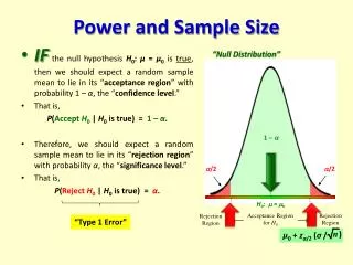
Buzzwords • Alpha (α) = P(Type I error) = P(Conclude experimental groups are different when they really are the same) • Beta () = P(Type II error) = P(Conclude the experimental groups are the same when they really are different) • Power = 1 - = P(Conclude experimental groups are different when they really are!)
Thoughts • When planning an experiment, one should determine a sample size that results in a statistical test powerful enough to declare significance for a reasonable difference in the means…if that difference truly exists in the population
Thoughts • Generally speaking...in order to calculate power/sample size, one needs a ‘guess’ about the pattern of the population means and an estimate of their variance • Otherwise the statistician feels that they have the role of dreaming up what the population means and variances are…YIKES!
Thoughts • α • 1- • Variance • Population means • N: • Represent the five items involved in power and sample size. • One needs to recognize that that you must input 4 of these items to get the fifth.
One or the other…. • Input ⇒ (α, 1- , variance,population means) ⇒ gives N • Input ⇒ (α, variance,population means, N) ⇒ gives 1- • One usually ends up iterating between the above to arrive at a sample size that has a desirable level of power.
How to Help Your Statistician Help You! • Usually a study has several questions to be answered…and a statistical test that goes with each. • Prioritize which of these are most important and arguably the ones power should be based on. • Organize your best bet on the population means and their variances…or some scenarios that are clinically important that you wish to detect (if they truly exist in the population).
How to Help Your Statistician Help You! • Determine what the resources of the study are…how many subjects can you afford. Communicate this up front. • Try to do some preliminary power calculations on your own. Its really fun!
Scenario 1 • Alpha =0.05, sigma=2 • |mu1 – mu2| = 2, that is, a two unit diff in means for a population • Propose n1 = 10 and n2 = 10
Noncentrality value =2.236, Critical value = |2.101| Table B.5, Values between 2.0 and 3.0, alpha = 0.05, df = 18 Power between 0.47 and 0.81, SAS calculation 0.56195
Now one has a couple of choices • Decide that a 2 unit difference in the means is reasonable and you can afford 30 subjects in each group
Noncentrality value =3.87, Critical value = |2.00| Table B.5, Values between 3.0 and 4.0, alpha = 0.05, df = 58 (60) Power between 0.84 and 0.98, SAS calculation 0.97044
Now one has a couple of choices • Decide that a 3 unit difference in the means is reasonable and you can only afford 10 subjects in each group
Noncentrality value =3.35 , Critical value = |2.101| Table B.5, Values between 3.0 and 4.0, alpha = 0.05, df = 18 Power between 0.81 and 0.97, SAS calculation 0.88621
Anova PowerF-dist Noncentrality Parameter r is the number of treatments
Anova Setting… • Suppose you have an experiment with 4 treatments (r =4) • Suppose mu1= 20, mu2 = 15, mu3 = 15, and mu4 = 12 • Suppose sigma = 4 • Suppose you can afford n = 5 in each group for a total of 20 subjects
Use table B.11 • r = 4, v1 = r –1 = 3, v2 = N – r = 20 – 4 = 16 • Alpha = 0.05 • Use phi = 1.6 • Power is between 0.6 and 0.86 • SAS calculation is 0.66052
Rejection Region F Distribution dfn = 3, dfd = 16, Alpha = 0.05, Critical value = 3.24
Area = 0.66052 Non Centrality parameter = 1.61 Power is area to the right of 3.24 on red F distribution
Suppose You’re Somewhat Clueless • Δ = max(mu) – min(mu) • Determine k = Δ/s.d. (‘effect size’) • Use table B.12 • Different levels of alpha = 0.2, 0.1. 0.05, and 0.01 • 1 – β = 0.7, 0.8, 0.9, and 0.95 • r : number of treatments, 2, 3, …., 10
From Our Earlier Anova Setting.. • mu1 = 20, mu2 = 15, mu3 = 15, mu4 = 12 • Δ = 20 – 12 = 8, sigma = 4 • K = Δ/sigma = 8/4 = 2 , r = 4