Mastering Image Filtering Techniques: A Computational Photography Guide
Delve into the world of image filtering in computational photography. Learn about pixels, image representation, filtering methods, hybrid images, and more. Explore various filters, spatial and frequency domains, and image pyramids. Understand linear filters, color image processing, and the power of Gaussian filters for smoothing and enhancement. Dive into practical examples and get hands-on experience with MATLAB and algebra tutorials. Enhance your skills and elevate your image processing abilities with this comprehensive guide.

Mastering Image Filtering Techniques: A Computational Photography Guide
E N D
Presentation Transcript
08/30/11 Pixels and Image Filtering Computational Photography Derek Hoiem Graphic: http://www.notcot.org/post/4068/
Administrative stuff • Any questions? • Matlab/algebra tutorial • Thursday (9/1): 5-6:30pm, SC 3403
Today’s Class: Pixels and Linear Filters • What is a pixel? How is an image represented? • What is image filtering and how do we do it? • Introduce Project 1: Hybrid Images
Next three classes • Image filters in spatial domain • Smoothing, sharpening, measuring texture • Image filters in the frequency domain • Denoising, sampling, image compression • Templates and Image Pyramids • Detection, coarse-to-fine registration
Digital camera A digital camera replaces film with a sensor array • Each cell in the array is light-sensitive diode that converts photons to electrons • Two common types: Charge Coupled Device (CCD) and CMOS • http://electronics.howstuffworks.com/digital-camera.htm Slide by Steve Seitz
Sensor Array CMOS sensor
Perception of Intensity from Ted Adelson
Perception of Intensity from Ted Adelson
Color Image R G B
Images in Matlab • Images represented as a matrix • Suppose we have a NxM RGB image called “im” • im(1,1,1) = top-left pixel value in R-channel • im(y, x, b) = y pixels down, x pixels to right in the bth channel • im(N, M, 3) = bottom-right pixel in B-channel • imread(filename) returns a uint8 image (values 0 to 255) • Convert to double format (values 0 to 1) with im2double column row R G B
Image filtering • Image filtering: compute function of local neighborhood at each position • Really important! • Enhance images • Denoise, resize, increase contrast, etc. • Extract information from images • Texture, edges, distinctive points, etc. • Detect patterns • Template matching
Example: box filter 1 1 1 1 1 1 1 1 1 Slide credit: David Lowe (UBC)
Image filtering 1 1 1 1 1 1 1 1 1 Credit: S. Seitz
Image filtering 1 1 1 1 1 1 1 1 1 Credit: S. Seitz
Image filtering 1 1 1 1 1 1 1 1 1 Credit: S. Seitz
Image filtering 1 1 1 1 1 1 1 1 1 Credit: S. Seitz
Image filtering 1 1 1 1 1 1 1 1 1 Credit: S. Seitz
Image filtering 1 1 1 1 1 1 1 1 1 ? Credit: S. Seitz
Image filtering 1 1 1 1 1 1 1 1 1 ? Credit: S. Seitz
Image filtering 1 1 1 1 1 1 1 1 1 Credit: S. Seitz
Box Filter 1 1 1 1 1 1 1 1 1 • What does it do? • Replaces each pixel with an average of its neighborhood • Achieve smoothing effect (remove sharp features) Slide credit: David Lowe (UBC)
Practice with linear filters 0 0 0 0 1 0 0 0 0 ? Original Source: D. Lowe
Practice with linear filters 0 0 0 0 1 0 0 0 0 Original Filtered (no change) Source: D. Lowe
Practice with linear filters 0 0 0 0 0 1 0 0 0 ? Original Source: D. Lowe
Practice with linear filters 0 0 0 0 0 1 0 0 0 Original Shifted left By 1 pixel Source: D. Lowe
Practice with linear filters 0 1 0 1 0 1 1 0 2 1 0 1 1 0 1 0 0 1 - ? (Note that filter sums to 1) Original Source: D. Lowe
Practice with linear filters 0 1 0 1 0 1 1 0 2 1 0 1 1 0 1 0 0 1 - Original • Sharpening filter • Accentuates differences with local average Source: D. Lowe
Sharpening Source: D. Lowe
Other filters 1 0 -1 2 0 -2 1 0 -1 Sobel Vertical Edge (absolute value)
Other filters Q? 1 2 1 0 0 0 -1 -2 -1 Sobel Horizontal Edge (absolute value)
How could we synthesize motion blur? theta = 30; len = 20; fil = imrotate(ones(1, len), theta, 'bilinear'); fil = fil / sum(fil(:)); figure(2), imshow(imfilter(im, fil));
Filtering vs. Convolution g=filter f=image • 2d filtering • h=filter2(g,f); or h=imfilter(f,g); • 2d convolution • h=conv2(g,f);
Key properties of linear filters Linearity: filter(f1 + f2) = filter(f1) + filter(f2) Shift invariance: same behavior regardless of pixel location filter(shift(f)) = shift(filter(f)) Any linear, shift-invariant operator can be represented as a convolution Source: S. Lazebnik
More properties • Commutative: a * b = b * a • Conceptually no difference between filter and signal • Associative: a * (b * c) = (a * b) * c • Often apply several filters one after another: (((a * b1) * b2) * b3) • This is equivalent to applying one filter: a * (b1 * b2 * b3) • Distributes over addition: a * (b + c) = (a * b) + (a * c) • Scalars factor out: ka * b = a * kb = k (a * b) • Identity: unit impulse e = [0, 0, 1, 0, 0],a * e = a Source: S. Lazebnik
Important filter: Gaussian • Weight contributions of neighboring pixels by nearness 0.003 0.013 0.022 0.013 0.003 0.013 0.059 0.097 0.059 0.013 0.022 0.097 0.159 0.097 0.022 0.013 0.059 0.097 0.059 0.013 0.003 0.013 0.022 0.013 0.003 5 x 5, = 1 Slide credit: Christopher Rasmussen
Gaussian filters • Remove “high-frequency” components from the image (low-pass filter) • Images become more smooth • Convolution with self is another Gaussian • So can smooth with small-width kernel, repeat, and get same result as larger-width kernel would have • Convolving two times with Gaussian kernel of width σ is same as convolving once with kernel of width σ√2 • Separable kernel • Factors into product of two 1D Gaussians Source: K. Grauman
Separability of the Gaussian filter Source: D. Lowe
Separability example * = = * 2D convolution(center location only) The filter factorsinto a product of 1Dfilters: Perform convolutionalong rows: Followed by convolutionalong the remaining column: Source: K. Grauman
Separability • Why is separability useful in practice?
Practical matters How big should the filter be? • Values at edges should be near zero • Rule of thumb for Gaussian: set filter half-width to about 3 σ
Practical matters • What is the size of the output? • MATLAB: filter2(g, f, shape) • shape = ‘full’: output size is sum of sizes of f and g • shape = ‘same’: output size is same as f • shape = ‘valid’: output size is difference of sizes of f and g full same valid g g g g f f f g g g g g g g g Source: S. Lazebnik