Pixels and Image Filtering
01/24/12. Pixels and Image Filtering. Computer Vision Derek Hoiem, University of Illinois. Graphic: http://www.notcot.org/post/4068/. Today’s Class: Pixels and Linear Filters. Review of lighting Reflection and absorption What is image filtering and how do we do it?

Pixels and Image Filtering
E N D
Presentation Transcript
01/24/12 Pixels and Image Filtering Computer Vision Derek Hoiem, University of Illinois Graphic: http://www.notcot.org/post/4068/
Today’s Class: Pixels and Linear Filters • Review of lighting • Reflection and absorption • What is image filtering and how do we do it? • Color models (if time allows)
Reflection models • Albedo: fraction of light that is reflected • Determines color (amount reflected at each wavelength) Very low albedo (hard to see shape) Higher albedo
Reflection models • Specular reflection: mirror-like • Light reflects at incident angle • Reflection color = incoming light color
Reflection models • Diffuse reflection • Light scatters in all directions (proportional to cosine with surface normal) • Observed intensity is independent of viewing direction • Reflection color depends on light color and albedo
Surface orientation and light intensity • Amount of light that hits surface from distant point source depends on angle between surface normal and source 1 2 prop to cosine of relative angle
Reflection models Lambertian: reflection all diffuse Mirrored: reflection all specular Glossy: reflection mostly diffuse, some specular Specularities
Questions • How many light sources are in the scene? • How could I estimate the color of the camera’s flash?
The plight of the poor pixel • A pixel’s brightness is determined by • Light source (strength, direction, color) • Surface orientation • Surface material and albedo • Reflected light and shadows from surrounding surfaces • Gain on the sensor • A pixel’s brightness tells us nothing by itself
Basis for interpreting intensity images • Key idea: for nearby scene points, most factors do not change much • The information is mainly contained in local differences of brightness
Next three classes: three views of filtering • Image filters in spatial domain • Filter is a mathematical operation of a grid of numbers • Smoothing, sharpening, measuring texture • Image filters in the frequency domain • Filtering is a way to modify the frequencies of images • Denoising, sampling, image compression • Templates and Image Pyramids • Filtering is a way to match a template to the image • Detection, coarse-to-fine registration
Image filtering • Image filtering: compute function of local neighborhood at each position • Linear filtering: function is a weighted sum/difference of pixel values • Really important! • Enhance images • Denoise, resize, increase contrast, etc. • Extract information from images • Texture, edges, distinctive points, etc. • Detect patterns • Template matching
Example: box filter 1 1 1 1 1 1 1 1 1 Slide credit: David Lowe (UBC)
Image filtering 1 1 1 1 1 1 1 1 1 Credit: S. Seitz
Image filtering 1 1 1 1 1 1 1 1 1 Credit: S. Seitz
Image filtering 1 1 1 1 1 1 1 1 1 Credit: S. Seitz
Image filtering 1 1 1 1 1 1 1 1 1 Credit: S. Seitz
Image filtering 1 1 1 1 1 1 1 1 1 Credit: S. Seitz
Image filtering 1 1 1 1 1 1 1 1 1 ? Credit: S. Seitz
Image filtering 1 1 1 1 1 1 1 1 1 ? Credit: S. Seitz
Image filtering 1 1 1 1 1 1 1 1 1 Credit: S. Seitz
Box Filter 1 1 1 1 1 1 1 1 1 • What does it do? • Replaces each pixel with an average of its neighborhood • Achieve smoothing effect (remove sharp features) Slide credit: David Lowe (UBC)
Practice with linear filters 0 0 0 0 1 0 0 0 0 ? Original Source: D. Lowe
Practice with linear filters 0 0 0 0 1 0 0 0 0 Original Filtered (no change) Source: D. Lowe
Practice with linear filters 0 0 0 0 0 1 0 0 0 ? Original Source: D. Lowe
Practice with linear filters 0 0 0 0 0 1 0 0 0 Original Shifted left By 1 pixel Source: D. Lowe
Practice with linear filters 0 1 0 1 0 1 1 0 2 1 0 1 1 0 1 0 0 1 - ? (Note that filter sums to 1) Original Source: D. Lowe
Practice with linear filters 0 1 0 1 0 1 1 0 2 1 0 1 1 0 1 0 0 1 - Original • Sharpening filter • Accentuates differences with local average Source: D. Lowe
Sharpening Source: D. Lowe
Other filters 1 0 -1 2 0 -2 1 0 -1 Sobel Vertical Edge (absolute value)
Other filters 1 2 1 0 0 0 -1 -2 -1 Sobel Horizontal Edge (absolute value)
Basic gradient filters 0 0 1 0 0 0 -1 -1 0 -1 0 0 0 0 1 1 1 0 0 0 -1 0 0 0 Horizontal Gradient Vertical Gradient or or
How could we synthesize motion blur? theta = 30; len = 20; fil = imrotate(ones(1, len), theta, 'bilinear'); fil = fil / sum(fil(:)); figure(2), imshow(imfilter(im, fil));
Filtering vs. Convolution g=filter f=image • 2d filtering • h=filter2(g,f); or h=imfilter(f,g); • 2d convolution • h=conv2(g,f);
Key properties of linear filters Linearity: filter(f1 + f2) = filter(f1) + filter(f2) Shift invariance: same behavior regardless of pixel location filter(shift(f)) = shift(filter(f)) Any linear, shift-invariant operator can be represented as a convolution Source: S. Lazebnik
More properties • Commutative: a * b = b * a • Conceptually no difference between filter and signal • Associative: a * (b * c) = (a * b) * c • Often apply several filters one after another: (((a * b1) * b2) * b3) • This is equivalent to applying one filter: a * (b1 * b2 * b3) • Distributes over addition: a * (b + c) = (a * b) + (a * c) • Scalars factor out: ka * b = a * kb = k (a * b) • Identity: unit impulse e = [0, 0, 1, 0, 0],a * e = a Source: S. Lazebnik
Important filter: Gaussian • Spatially-weighted average 0.003 0.013 0.022 0.013 0.003 0.013 0.059 0.097 0.059 0.013 0.022 0.097 0.159 0.097 0.022 0.013 0.059 0.097 0.059 0.013 0.003 0.013 0.022 0.013 0.003 5 x 5, = 1 Slide credit: Christopher Rasmussen
Gaussian filters • Remove “high-frequency” components from the image (low-pass filter) • Images become more smooth • Convolution with self is another Gaussian • So can smooth with small-width kernel, repeat, and get same result as larger-width kernel would have • Convolving two times with Gaussian kernel of width σ is same as convolving once with kernel of width σ√2 • Separable kernel • Factors into product of two 1D Gaussians Source: K. Grauman
Separability of the Gaussian filter Source: D. Lowe
Separability example * = = * 2D filtering(center location only) The filter factorsinto a product of 1Dfilters: Perform filteringalong rows: Followed by filteringalong the remaining column: Source: K. Grauman
Separability • Why is separability useful in practice?
Practical matters How big should the filter be? • Values at edges should be near zero important! • Rule of thumb for Gaussian: set filter half-width to about 3 σ
Practical matters • What about near the edge? • the filter window falls off the edge of the image • need to extrapolate • methods: • clip filter (black) • wrap around • copy edge • reflect across edge Source: S. Marschner