Image Filtering
Image Filtering. CS485/685 Computer Vision Prof. George Bebis. What is image filtering?. f(x,y). g(x,y). filtering. filtering. Image Filtering Methods. Spatial Domain Frequency Domain (i.e., uses Fourier Transform). Spatial Domain Methods. g(x,y). f(x,y). f(x,y). g(x,y).

Image Filtering
E N D
Presentation Transcript
Image Filtering CS485/685 Computer Vision Prof. George Bebis
What is image filtering? f(x,y) g(x,y) filtering filtering
Image Filtering Methods • Spatial Domain • Frequency Domain (i.e., uses Fourier Transform)
Spatial Domain Methods g(x,y) f(x,y) f(x,y) g(x,y)
Point Processing Methods • Convert a given pixel value to a new pixel value based on some predefined function.
Point Processing Methods - Examples Negative Contrast stretching Thresholding Histogram Equalization
output image Area Processing Methods • Need to define: • Area shape and size (2) Operation
Area Shape and Size • Area shape is typically defined using a rectangular mask. • Area size is determined by mask size. • e.g., 3x3 or 5x5 • Mask size is an important parameter!
Operation • Typically linear combinations of pixel values. • e.g., weight pixel values and add them together. • Different results can be obtained using different weights. • e.g., smoothing, sharpening, edge detection). mask
0 0 0 0 0.5 0 0 0.5 10 5 3 4 8 6 1 1 1 8 Example 1 Local image neighborhood mask Modified image data
Common Linear Operations • Correlation • Convolution
h(i,j) g(i,j) f(i,j) Correlation • A filtered image is generated as the center of the mask visits every pixel in the input image. n x n mask filtered image
Handling Pixels Close to Boundaries wrap around pad with zeroes 0 0 0 ……………………….0 or 0 0 0 ……………………….0
x θ y Geometric Interpretation of Correlation • Suppose x and y are two n-dimensional vectors: • The dot product of x with y is defined as: • Correlation generalizes the notion of dot product using vector notation:
Geometric Interpretation of Correlation (cont’d) cos(θ) measures the similarity between x and y • Normalized correlation (i.e., divide by lengths)
Normalized Correlation • Measure the similarity between images or parts of images. mask =
Normalized Correlation (cont’d) • Traditional correlation cannot handle changes due to: • size • orientation • shape (e.g., deformable objects). ?
Convolution • Same as correlation except that the mask is flipped, both horizontally and vertically. V H Notation: For symmetric masks (i.e., h(i,j)=h(-i,-j)), convolution is equivalent to correlation! h * f = f * h
Correlation/Convolution Examples Correlation: Convolution:
1st derivative of Gaussian 2nd derivative of Gaussian Gaussian How do we choose the mask weights? • Depends on the application. • Usually by sampling certain functions and their derivatives. Good for image smoothing Good for image sharpening
Normalization of Mask Weights • Sum of weights affects overall intensity of output image. • Positive weights • Normalize them such that they sum to one. • Both positive and negative weights • Should sum to zero(but not always) 1/9 1/16
Smoothing Using Averaging • Idea: replace each pixel by the average of its neighbors. • Useful for reducing noise and unimportant details. • The size of the mask controls the amount of smoothing.
Smoothing Using Averaging (cont’d) • Trade-off: noise vs blurring and loss of detail. original 3x3 5x5 7x7 15x15 25x25
Gaussian Smoothing • Idea: replace each pixel by a weighted average of its neighbors • Mask weights are computed by sampling a Gaussian function Note: weight values decrease with distance from mask center!
Gaussian Smoothing (cont’d) mask size depends on σ : • σ determines the degree of smoothing! σ=3
Gaussian Smoothing (cont’d) Gaussian(sigma, hSize, h) float sigma, *h; inthSize; { inti; float cst, tssq, x, sum; cst = 1./(sigma*sqrt(2.0*PI)) ; tssq = 1./(2*sigma*sigma) ; for(i=0; i<hSize; i++) { x=(float)(i-hSize/2); h[i]=(cst*exp(-(x*x*tssq))) ; } // normalize sum=0.0; for(i=0;i<hSize;i++) sum += h[i]; for(i=0;i<hSize;i++) h[i] /= sum; } halfSize=(int)(2.5*sigma); hSize=2*halfSize; if (hSize % 2 == 0) ++hSize; // odd size
Gaussian Smoothing - Example = 1 pixel = 10 pixels = 30 pixels = 5 pixels
Averaging vs Gaussian Smoothing Averaging Gaussian
Properties of Gaussian Convolution with self is another Gaussian Special case: convolving two times with Gaussian kernel of width is equivalent to convolving once with kernel of width * =
Properties of Gaussian (cont’d) • Separable kernel: a 2D Gaussian can be expressed as the product of two 1D Gaussians.
Properties of Gaussian (cont’d) • 2D Gaussian convolution can be implemented more efficiently using 1D convolutions:
row get a new image Ir Convolve each column of Ir with g Properties of Gaussian (cont’d)
Example * = = * 2D convolution(center location only) O(n2) The filter factorsinto a product of 1Dfilters: Perform convolutionalong rows: O(2n)=O(n) Followed by convolutionalong the remaining column:
1st derivative of Gaussian Image Sharpening • Idea: compute intensity differences in local image regions. • Useful for emphasizing transitions in intensity (e.g., in edge detection).