Binary Encoding
This document outlines the process of computing spectral means for pixel samples and binary encoding for enhanced feature extraction in spectral analysis. By assigning values based on the spectral mean, the method allows effective comparison while minimizing sensitivity to illumination variations. The presented system includes continuum definition, feature computation, and hierarchical classification to optimize library spectra. The output features quantitative abundance maps and improves analysis accuracy, addressing noise and ensuring robustness in spectral representation.

Binary Encoding
E N D
Presentation Transcript
Binary Encoding Compute spectral mean of sample (pixel) assign a 1 to bands equal or greater than mean and 0 to those less than mean. Easy to store very rapid to do comparison. Sensitive to band structure and relatively insensitive to slope and illumination variations. Note the probability of match can be plotted as brightness based on % of binary vector match. In many cases, only one or more spectral regions are compared to avoid regions of little spectral character causing significant mismatch. May need to smooth noisy spectra first to reduce random fluctuations. Binary Encoding
Expert System Automated feature extraction • Apply to library and image features after calibration to reflectance 1. Define continuum -locate high points and straight line fit between them see Figure 13a 2. Divide spectrum by continuum (see Figure 13b) Binary Encoding
3. Compute minimums and select 10 strongest features 4. Compute position (l), band depth, FWHM and asymmetry - asymmetry is Ln ( of reflective channels to right of minimum/ of reflectance channels to left) see Figure 13c Binary Encoding
N.B. not clear if he is using # of channels or value of reflectance. # of channels seem cleaner • Rules were built with a hierarchical classifier to classify library spectra. • The results of expert and binary encoding were combined in the expert. see Figure 16 Binary Encoding
* In practice expert not used in a hierarchy but as probability of prediction. Features arbitrarily weighted by 1 must have, 0.6 should have, 0.3 may have It appears as though only presence or absence of absorption features were used (i.e., feature in probe estimate is either 0 or 1. Final prob = 0.67 probe + 0.33 probb where probb is the probability estimate from the binary feature match. The inclusion of probb was very helpful for noisy spectra. N.B. neither of these are true probabilities! Binary Encoding
Output - Continuum removed “reflectance spectra” (cube) - feature cube (l, depth, FWHM, asym for 10 strongest features) - analysis cube: 1) (prob estimate for each entry in library (25 library values in this case) cf. Fig 18 2) material map of most likely material 3) of probabilities map 4) # of prob > 0.5 (mixed pixels?) 5) no prob > 0.1 (unknown) Binary Encoding
They go on to use classic unconstrained and fully constrained unmixing of most likely materials ( 5) to generate quantitative abundance maps! N.B. used image derived end members. They point out the importance of error images from unmixing to highlight missing spectra from library. The expert is designed to reduce the library from tens or hundreds of spectra to a few to give to unmixing. Although not specified in the paper, it would be reasonable to include a different small set of features for each pixel in the unmixing process. In the unconstrained case fraction maps, sum of fractions and error images were produced. The sum of fractions error images were used to point out errors. Binary Encoding