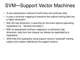
SVM — Support Vector Machines
SVM — Support Vector Machines. A new classification method for both linear and nonlinear data It uses a nonlinear mapping to transform the original training data into a higher dimension With the new dimension, it searches for the linear optimal separating hyperplane (i.e., “decision boundary”)

SVM — Support Vector Machines
E N D
Presentation Transcript
SVM—Support Vector Machines • A new classification method for both linear and nonlinear data • It uses a nonlinear mapping to transform the original training data into a higher dimension • With the new dimension, it searches for the linear optimal separating hyperplane (i.e., “decision boundary”) • With an appropriate nonlinear mapping to a sufficiently high dimension, data from two classes can always be separated by a hyperplane • SVM finds this hyperplane using support vectors (“essential” training tuples) and margins (defined by the support vectors)
SVM—History and Applications • Vapnik and colleagues (1992)—groundwork from Vapnik & Chervonenkis’ statistical learning theory in 1960s • Features: training can be slow but accuracy is high owing to their ability to model complex nonlinear decision boundaries (margin maximization) • Used both for classification and prediction • Applications: • handwritten digit recognition, object recognition, speaker identification, benchmarking time-series prediction tests
SVM—Linearly Separable • A separating hyperplane can be written as W ● X + b = 0 where W={w1, w2, …, wn} is a weight vector and b a scalar (bias) • For 2-D it can be written as w0 + w1 x1 + w2 x2 = 0 • The hyperplane defining the sides of the margin: H1: w0 + w1 x1 + w2 x2 ≥ 1 for yi = +1, and H2: w0 + w1 x1 + w2 x2 ≤ – 1 for yi = –1 • Any training tuples that fall on hyperplanes H1 or H2 (i.e., the sides defining the margin) are support vectors • This becomes a constrained (convex) quadratic optimization problem: Quadratic objective function and linear constraints Quadratic Programming (QP) Lagrangian multipliers
Support vectors • The support vectors define the maximum margin hyperplane! • All other instances can be deleted without changing its position and orientation • This means the hyperplane can be written as
Finding support vectors • Support vector: training instance for which i > 0 • Determine i and b ?—A constrainedquadratic optimization problem • Off-the-shelf tools for solving these problems • However, special-purpose algorithms are faster • Example: Platt’s sequential minimal optimization algorithm (implemented in WEKA) • Note: all this assumes separable data!
Extending linear classification • Linear classifiers can’t model nonlinear class boundaries • Simple trick: • Map attributes into new space consisting of combinations of attribute values • E.g.: all products of n factors that can be constructed from the attributes • Example with two attributes and n = 3:
Nonlinear SVMs • “Pseudo attributes” represent attribute combinations • Overfitting not a problem because the maximum margin hyperplane is stable • There are usually few support vectors relative to the size of the training set • Computation time still an issue • Each time the dot product is computed, all the “pseudo attributes” must be included
A mathematical trick • Avoid computing the “pseudo attributes”! • Compute the dot product before doing the nonlinear mapping • Example: forcompute • Corresponds to a map into the instance space spanned by all products of n attributes
Other kernel functions • Mapping is called a “kernel function” • Polynomial kernel • We can use others: • Only requirement: • Examples:
Problems with this approach • 1st problem: speed • 10 attributes, and n = 5 >2000 coefficients • Use linear regression with attribute selection • Run time is cubic in number of attributes • 2nd problem: overfitting • Number of coefficients is large relative to the number of training instances • Curse of dimensionality kicks in
Sparse data • SVM algorithms speed up dramatically if the data is sparse (i.e. many values are 0) • Why? Because they compute lots and lots of dot products • Sparse data compute dot products very efficiently • Iterate only over non-zero values • SVMs can process sparse datasets with 10,000s of attributes
Applications • Machine vision: e.g face identification • Outperforms alternative approaches (1.5% error) • Handwritten digit recognition: USPS data • Comparable to best alternative (0.8% error) • Bioinformatics: e.g. prediction of protein secondary structure • Text classifiation • Can modify SVM technique for numeric prediction problems