Feedforward Neural Networks. Classification and Approximation
Feedforward Neural Networks. Classification and Approximation. Classification and Approximation Problems BackPropagation (BP) Neural Networks Radial Basis Function (RBF) Networks Support Vector Machines. Classification problems. Example 1 : identifying the type of an iris flower.


Feedforward Neural Networks. Classification and Approximation
E N D
Presentation Transcript
Feedforward Neural Networks. Classification and Approximation • Classification and Approximation Problems • BackPropagation (BP) Neural Networks • Radial Basis Function (RBF) Networks • Support Vector Machines Neural and Evolutionary Computing - Lecture 2-3
Classification problems Example 1:identifying the type of an iris flower • Attributes: sepal/petal lengths, sepal/petal width • Classes: Iris setosa, Iris versicolor, Iris virginica Example 2:handwritten character recognition • Attributes: various statistical and geometrical characteristics of the corresponding image • Classes: set of characters to be recognized • Classification = find the relationship between some vectors with attribute values and classes labels (Du Trier et al; Feature extraction methods for character Recognition. A Survey. Pattern Recognition, 1996) Neural and Evolutionary Computing - Lecture 2-3 2
Classification problems Classification: • Problem: identify the class to which a given data (described by a set of attributes) belongs • Prior knowledge: examples of data belonging to each class Simple example: linearly separable case A more difficult example: nonlinearly separable case Neural and Evolutionary Computing - Lecture 2-3
Approximation problems • Estimation of a hous price knowing: • Total surface • Number of rooms • Size of the back yard • Location => approximation problem = find a numerical relationship between some output and input value(s) • Estimating the amount of resources required by a software application or the number of users of a web service or a stock price knowing historical values => prediction problem= find a relationship between future values and previous values Neural and Evolutionary Computing - Lecture 2-3
Approximation problems Regression (fitting, prediction): • Problem: estimate the value of a characteristic depending on the values of some predicting characteristics • Prior knowledge: pairs of corresponding values (training set) y Estimated value (for x’ which is not in the training set) Known values x’ x Neural and Evolutionary Computing - Lecture 2-3
Approximation problems All approximation (mapping) problems can be stated as follows: Starting from a set of data (Xi,Yi), Xi in RN and Yi din RM find a function F:RN -> RM which minimizes the distance between the data and the corresponding points on its graph: ||Yi-F(Xi)||2 Questions: • What structure (shape) should have F ? • How can we find the parameters defining the properties of F ? Neural and Evolutionary Computing - Lecture 2-3
Approximation problems Can be such a problem be solved by using neural networks ? Yes, at least in theory,the neural networks are proven “universal approximators” [Hornik, 1985]: “ Any continuous function can be approximated by a feedforward neural network having at least one hidden layer. The accuracy of the approximation depends on the number of hidden units.” • The shape of the function is influenced by the architecture of the network and by the properties of the activation functions. • The function parameters are in fact the weights corresponding to the connections between neurons. Neural and Evolutionary Computing - Lecture 2-3
Neural Networks Design Steps to follow in designing a neural network: • Choose the architecture: number of layers, number of units on each layer, activation functions, interconnection style • Train the network: compute the values of the weights using the training set and a learning algorithm. • Validate/test the network: analyze the network behavior for data which do not belong to the training set. Neural and Evolutionary Computing - Lecture 2-3
Functional units (neurons) inputs y1 Functional unit: several inputs, one output Notations: • input signals: y1,y2,…,yn • synaptic weights: w1,w2,…,wn (they model the synaptic permeability) • threshold (bias): b (or theta) (it models the activation threshold of the neuron) • Output: y • All these values are usually real numbers w1 output y2 w2 yn wn Weights assigned to the connections Neural and Evolutionary Computing - Lecture 2-3
Functional units (neurons) Output signal generation: • The input signals are “combined” by using the connection weights and the threshold • The obtained value corresponds to the local potential of the neuron • This “combination” is obtained by applying a so-called aggregation function • The output signal is constructed by applying an activation function • It corresponds to the pulse signals propagated along the axon Neuron’s state (u) Output signal (y) Input signals (y1,…,yn) Aggregation function Activation function Neural and Evolutionary Computing - Lecture 2-3
Functional units (neurons) Weighted sum Euclidean distance Aggregation functions: Multiplicative neuron High order connections Remark: in the case of the weighted sum the threshold can be interpreted as a synaptic weight which corresponds to a virtual unit which always produces the value -1 Neural and Evolutionary Computing - Lecture 2-3
Functional units (neurons) Activation functions: signum Heaviside Saturated linear linear Neural and Evolutionary Computing - Lecture 2-3
Functional units (neurons) (Hyperbolic tangent) Sigmoidal aggregation functions (Logistic) Neural and Evolutionary Computing - Lecture 2-3
Functional units (neurons) -1 b x1 w1 OR • What can do a single neuron ? • It can solve simple problems (linearly separable problems) 0 1 y 0 1 1 1 w2 0 1 x2 y=H(w1x1+w2x2-b) Ex: w1=w2=1, w0=0.5 Neural and Evolutionary Computing - Lecture 2-3
Functional units (neurons) -1 w0 x1 w1 OR • What can do a single neuron ? • It can solve simple problems (linearly separable problems) 0 1 y 0 1 1 1 w2 0 1 x2 y=H(w1x1+w2x2-w0) Ex: w1=w2=1, w0=0.5 AND 0 1 0 0 0 1 0 1 y=H(w1x1+w2x2-w0) Ex: w1=w2=1, w0=1.5 Neural and Evolutionary Computing - Lecture 2-3
Functional units (neurons) Representation of boolean functions: f:{0,1}2->{0,1} Linearly separable problem: one layer network OR Nonlinearly separable problem: multilayer network XOR Neural and Evolutionary Computing - Lecture 2-3
Architecture and notations Input layer Hidden layers Output layer Feedforward network with K layers 0 1 k Wk W1 W2 Wk+1 WK … K … Xk Yk Fk XK YK FK Y0=X X1 Y1 F1 X = input vector, Y= output vector, F=vectorial activation function Neural and Evolutionary Computing - Lecture 2-3
Functioning Computation of the output vector FORWARD Algorithm (propagation of the input signal toward the output layer) Y[0]:=X (X is the input signal) FOR k:=1,K DO X[k]:=W[k]Y[k-1] Y[k]:=F(X[k]) ENDFOR Rmk: Y[K] is the output of the network Neural and Evolutionary Computing - Lecture 2-3
A particular case One hidden layer Adaptive parameters: W1, W2 Neural and Evolutionary Computing - Lecture 2-3
Learning process Learning based on minimizing a error function • Training set: {(x1,d1), …, (xL,dL)} • Error function (mean squared error): • Aim of learning process: find W which minimizes the error function • Minimization method: gradient method Neural and Evolutionary Computing - Lecture 2-3
Learning process Gradient based adjustement Learning rate xk yk xi yi El(W) Neural and Evolutionary Computing - Lecture 2-3
Learning process • Partial derivatives computation xk yk xi yi Neural and Evolutionary Computing - Lecture 2-3
Learning process • Partial derivatives computation Remark: The derivatives of sigmoidal activation functions have particular properties: Logistic: f’(x)=f(x)(1-f(x)) Tanh: f’(x)=1-f2(x) Neural and Evolutionary Computing - Lecture 2-3
The BackPropagation Algorithm Computation of the error signal (BACKWARD) Main idea: For each example in the training set: - compute the output signal - compute the error corresponding to the output level - propagate the error back into the network and store the corresponding delta values for each layer - adjust each weight by using the error signal and input signal for each layer Computation of the output signal (FORWARD) Neural and Evolutionary Computing - Lecture 2-3
The BackPropagation Algorithm Rmk. • The weights adjustment depends on the learning rate • The error computation needs the recomputation of the output signal for the new values of the weights • The stopping condition depends on the value of the error and on the number of epochs • This is a so-called serial (incremental) variant: the adjustment is applied separately for each example from the training set General structure Random initialization of weights REPEAT FOR l=1,L DO FORWARD stage BACKWARD stage weights adjustement ENDFOR Error (re)computation UNTIL <stopping condition> epoch Neural and Evolutionary Computing - Lecture 2-3
The BackPropagation Algorithm Details (serial variant) Neural and Evolutionary Computing - Lecture 2-3
The BackPropagation Algorithm Details (serial variant) E* denotes the expected training accuracy pmax denots the maximal number of epochs Neural and Evolutionary Computing - Lecture 2-3
The BackPropagation Algorithm Rmk. • The incremental variant can be sensitive to the presentation order of the training examples • The batch variant is not sensitive to this order and is more robust to the errors in the training examples • It is the starting algorithm for more elaborated variants, e.g. momentum variant Batch variant Random initialization of weights REPEAT initialize the variables which will contain the adjustments FOR l=1,L DO FORWARD stage BACKWARD stage cumulate the adjustments ENDFOR Apply the cumulated adjustments Error (re)computation UNTIL <stopping condition> epoch Neural and Evolutionary Computing - Lecture 2-3
The BackPropagation Algorithm Details (batch variant) Neural and Evolutionary Computing - Lecture 2-3
The BackPropagation Algorithm Neural and Evolutionary Computing - Lecture 2-3
Variants Different variants of BackPropagation can be designed by changing: • Error function • Minimization method • Learning rate choice • Weights initialization Neural and Evolutionary Computing - Lecture 2-3
Error function: MSE (mean squared error function) is appropriate in the case of approximation problems For classification problems a better error function is the cross-entropy error: Particular case: two classes (one output neuron): dl is from {0,1} (0 corresponds to class 0 and 1 corresponds to class 1) yl is from (0,1) and can be interpreted as the probability of class 1 Variants Rmk: the partial derivatives change, thus the adjustment terms will be different Neural and Evolutionary Computing - Lecture 2-3
Variants Entropy based error: • Different values of the partial derivatives • In the case of logistic activation functions the error signal will be: Neural and Evolutionary Computing - Lecture 2-3
Variants Minimization method: • The gradient method is a simple but not very efficient method • More sophisticated and faster methods can be used instead: • Conjugate gradient methods • Newton’s method and its variants • Particularities of these methods: • Faster convergence (e.g. the conjugate gradient converges in n steps for a quadratic error function) • Needs the computation of the hessian matrix (matrix with second order derivatives) : second order methods Neural and Evolutionary Computing - Lecture 2-3
Variants Example: Newton’s method Neural and Evolutionary Computing - Lecture 2-3
Variants Particular case: Levenberg-Marquardt • This is the Newton method adapted for the case when the objective function is a sum of squares (as MSE is) Used in order to deal with singular matrices Advantage: • Does not need the computation of the hessian Neural and Evolutionary Computing - Lecture 2-3
Problems in BackPropagation • Low convergence rate (the error decreases too slow) • Oscillations (the error value oscillates instead of continuously decreasing) • Local minima problem (the learning process is stuck in a local minima of the error function) • Stagnation (the learning process stagnates even if it is not a local minima) • Overtraining and limited generalization Neural and Evolutionary Computing - Lecture 2-3
Problems in BackPropagation Problem 1: The error decreases too slow or the error value oscillates instead of continuously decreasing Causes: • Inappropriate value of the learning rate (too small values lead to slow convergence while too large values lead to oscillations) • Solution: adaptive learning rate • Slow minimization method (the gradient method needs small learning rates in order to converge) Solutions: - heuristic modification of the standard BP (e.g. momentum) - other minimization methods (Newton, conjugate gradient) Neural and Evolutionary Computing - Lecture 2-3
Problems in BackPropagation Adaptive learning rate: • If the error is increasing then the learning rate should be decreased • If the error significantly decreases then the learning rate can be increased • In all other situations the learning rate is kept unchanged Example: γ=0.05 Neural and Evolutionary Computing - Lecture 2-3
Problems in BackPropagation Momentum variant: • Increase the convergence speed by introducing some kind of “inertia” in the weights adjustment: the weight changes corresponding to the current epoch includes the adjustments from the previous epoch Momentum coefficient:α in [0.1,0.9] Neural and Evolutionary Computing - Lecture 2-3
Problems in BackPropagation Momentum variant: • The effect of these enhancements is that flat spots of the error surface are traversed relatively rapidly with a few big steps, while the step size is decreased as the surface gets rougher. This implicit adaptation of the step size increases the learning speed significantly. Simple gradient descent Use of inertia term Neural and Evolutionary Computing - Lecture 2-3
Problems in BackPropagation Problem 2: Local minima problem (the learning process is stuck in a local minima of the error function) Cause: the gradient based methods are local optimization methods Solutions: • Restart the training process using other randomly initialized weights • Introduce random perturbations into the values of weights: • Use a global optimization method Neural and Evolutionary Computing - Lecture 2-3
Problems in BackPropagation Solution: • Replacing the gradient method with a stochastic optimization method • This means using a random perturbation instead of an adjustment based on the gradient computation • Adjustment step: Rmk: • The adjustments are usually based on normally distributed random variables • If the adjustment does not lead to a decrease of the error then it is not accepted Neural and Evolutionary Computing - Lecture 2-3
Problems in BackPropagation Problem 3: Stagnation (the learning process stagnates even if it is not a local minima) Cause: the adjustments are too small because the arguments of the sigmoidal functions are too large Solutions: • Penalize the large values of the weights (weights-decay) • Use only the signs of derivatives not their values Very small derivates Neural and Evolutionary Computing - Lecture 2-3
Problems in BackPropagation Penalization of large values of the weights: add a regularization term to the error function The adjustment will be: Neural and Evolutionary Computing - Lecture 2-3
Problems in BackPropagation Resilient BackPropagation (use only the sign of the derivative not its value) Neural and Evolutionary Computing - Lecture 2-3
Problems in BackPropagation Problem 4: Overtraining and limited generalization ability 10 hidden units 5 hidden units Neural and Evolutionary Computing - Lecture 2-3
Problems in BackPropagation Problem 4: Overtraining and limited generalization ability 20 hidden units 10 hidden units Neural and Evolutionary Computing - Lecture 2-3
Problems in BackPropagation Problem 4: Overtraining and limited generalization ability Causes: • Network architecture (e.g. number of hidden units) • A large number of hidden units can lead to overtraining (the network extracts not only the useful knowledge but also the noise in data) • The size of the training set • Too few examples are not enough to train the network • The number of epochs (accuracy on the training set) • Too many epochs could lead to overtraining Solutions: • Dynamic adaptation of the architecture • Stopping criterion based on validation error; cross-validation Neural and Evolutionary Computing - Lecture 2-3
Problems in BackPropagation Dynamic adaptation of the architectures: • Incrementalstrategy: • Start with a small number of hidden neurons • If the learning does not progress new neurons are introduced • Decremental strategy: • Start with a large number of hidden neurons • If there are neurons with small weights (small contribution to the output signal) they can be eliminated Neural and Evolutionary Computing - Lecture 2-3