Pseudoinverse Learning Algorithm for Feedforward Neural Networks
This presentation discusses the Pseudoinverse Learning Algorithm for improving the training of Feedforward Neural Networks (FNNs), which are valuable for pattern classification and function approximation. Traditional backpropagation suffers from problems such as slow convergence rates and local minima. Our proposed algorithm enhances training efficiency by using batch processing and matrix operations. Furthermore, it explores the existence of pseudoinverse solutions to minimize error functions, presenting numerical examples and results from real-world applications, including software reliability models. ###

Pseudoinverse Learning Algorithm for Feedforward Neural Networks
E N D
Presentation Transcript
Pseudoinverse Learning Algorithm for Feedforward Neural Networks Supervisor: Professor Michael Lyu Guo, Ping Markers: Professor L.W. Chan and I. King Department of Computer Science & Engineering, The Chinese University of Hong Kong, Hong Kong September 21, 2014
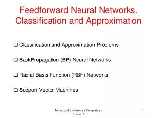
Introduction • Feedforward Neural Network • Widely used for pattern classification and universal approximation • Supervised learning task • Back propagation algorithm used to train the neural network • Poor convergence rate and local minima problem • Learning factors problem ( learning rate, momentum constant) • Time-consuming computation for some task by BP • Pseudoinverse Learning Algorithm • Batch-way learning • Matrix inner product and pseudoinverse operation
Network Structure (a) • Multilayer Neural Network (Mathematics Expression) • Input matrix: , output matrix: • Connect weight matrix • Nonlinear activate function • Network Mapping Function (with two hidden layers)
Network Structure (b) • Multilayer Neural Network (Mathematics Expression) • Denote l-th layer output • Network output: • To find the weigh matrices based on training data set
Pseudoinverse Solution (a) • Existence of the Solution • Linear Algebra Theorem: • Best Approximation Solution (Theorem) • The best solution for is • Pseudoinverse solution
Pseudoinverse Solution (b) • Minimize error function • Learning Task • If Y is full rank, above equation will be held • Learning task becomes to raise the rank of Y.
Pseudoinverse Learning Algorithm • Let • Compute • Yes, go to 6. No, next step • Let feed this as input to next layer, compute • Compute and go to step 3 • Let • Stop training. Real network output is
Add and Delete Sample (b) Computation efficiently Griville’s Theorem Add a sample: From (k-1)-th to calculate k-th pseudoinverse matrix
Add and Delete Sample (b) Computation efficiently Delete a sample: Let Bordering algorithm: Delete a sample: From (k+1)-th to calculate k-th pseudoinverse matrix
Numerical Examples (a) Function Mapping (1) Sin(x) (smooth function) (2) Nonlinear function: 8-D input, 3-D output (3) Smooth function (4) Piecewise smooth function
Numerical Examples (b) Function Mapping Table 1 Generalization ability test results. 20 training samples, 100 test samples Table 2 Generalization ability test results. 5 or 50 training samples, 100 test samples
o o o o o * o * o 1.5 o o o o o * 1 o o o o * o o o o o o o o o o * * o o o o o o * o * o o o o o o o o * o o o o o o o o * o o o * * o o o 1 o o o o 0.5 o o o * o o o o o o o o o o * o * o o o o o * o o o o o o * * o o o o o o * o o Output o 0.5 o o o Output o o * * 0 o o o o o o o o * o o o o o * o * o o o o o o o o * o * o o o o o o o o o o o o o o o o o o * o o o o * o 0 o * o o o o * o o -0.5 o o o o o o o * o * o o o o o o o * o o o * o o o o o o o o o o * o * o o * o -0.5 o o o o * o o o o o * o o o o o o o o * -1 0 0.5 1 1.5 2 2.5 3 0 1 2 3 4 5 6 Input Input o o o o o o o o o o o 1.5 * * o o o o o o 1.5 o o o o o o o * o o o o o o o o o o o * o o o o o o o o o o o o o * o 1 o 1 o o o o * o o o o o o o o o * o o o o o o o o o o o o o o o * o 0.5 o o o o o 0.5 o o o o * o o o o o o o o o o * o o o o o o Output * * 0 o Output * * * 0 o o o * o o o o o o o o o o * o o o o o o o o o * -0.5 -0.5 o o o o o o o * o o o o o * o o o o o o o o * -1 o -1 o o o o o o o o o o o o o * o o o o o o o o o o o o o o * o o o o o o o o o o o -1.5 o o * o o -1.5 o o o o o * o o o o o 0 1 2 3 4 5 6 0 1 2 3 4 5 6 Input Input Numerical Examples (c) Function Mapping “*”— training data, “o”– test data Example 1 Example 3 Example 4, 20 training samples Example 4, 5 training samples
* 1 * * * o * * o o * * 0.8 o * * o failures o o o * * 0.6 * o * * * * * * of * 0.4 o o * * * o * * o * Number * o * 0.2 * * * * * * * * o * 0 o 0 0.2 0.4 0.6 0.8 1 Execution Time Numerical Examples (d) Real world data set Software reliability growth model -- Sys1 data Total 54 samples, partitioned data into training samples (37) and test samples (17). “*”— training data, “o”– test data
+ + + + 1 + + + o + 0.8 failures o 0.6 + of o 0.4 o o o o o o o o Number o 0.2 o + + o o + + + + + o 0 0 0.2 0.4 0.6 0.8 1 Execution Time Numerical Examples (e) Real world data set Software reliability growth model -- Sys1 data Stacked generalization test, level-0 output is the level-1 input. “o”— level-0 output, “+”– level-1 output. Generalization is poor
Discussion • Local minima can be avoided by certain initialization. • No user selected parameter, “learning factor” problem is avoided. • Differentiable activate function is not necessary • Batch way learning, speed is fast • Provide an effective method to investigate some computation-intensive techniques • Further work: to find the techniques for generalization when noise data presented.
Thanks End of Presentation Q & A September 21, 2014